
Illustrates how to set up a grid of points to monitor the maximum amplitude of the wave at each point on a grid of points, a transect, and a curve along the shoreline.
This uses the "fgmax" (fixed grid maxima monitoring) capabilities described in http://www.clawpack.org/fgmax.html.
To test:
python make_fgmax.py   # to create fgmax_grid.txt
make .output
python plot_fgmax.py   # to plot fgmax results
make plots
Or simply:
make all
In addition to the usual time frame plots in _plots, this should produce
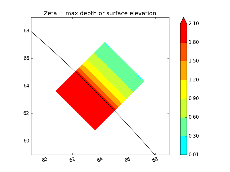
_plots/fgmax_grid1.png, maximum depth on an fgmax grid near the shoreline (black curve) along the x-axis.
_plots/fgmax_grid2.png, maximum depth on an fgmax grid near the shoreline (black curve) along the diagonal.
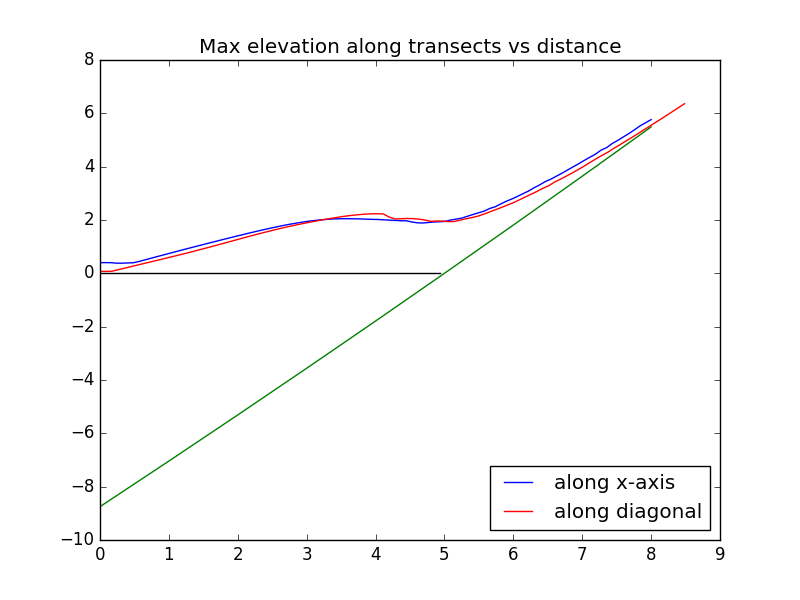
_plots/fgmax_transects.png, maximum surface elevation on a transect orthogonal to shoreline. Two transects are shown, one at the x-axis and the other along the diagonal.
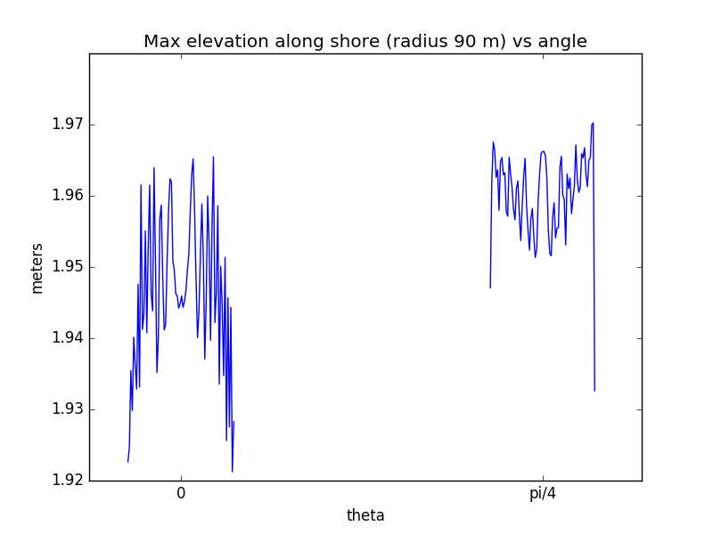
_plots/fgmax_along_shore.png, maximum surface elevation = depth at the shoreline (located at radius r = 90 meters) as a function of theta. The max values are only monitored on refinement level 3, which is only allowed near the x-axis and the diagonal, so intermediate values of theta show no results.
Due to radial symmetry the maximum depth should be independent of theta, and this plot should show that the value is around 1.95±0.03 meters.
Note:
This example is based on $CLAW/geoclaw/examples/tsunami/bowl-radial but with some changes to parameters and the topography is adjusted so the shoreline is at radius 90 meters.
See http://www.clawpack.org/fgmax.html for more information about specifying fgmax parameters.
The file make_fgmax.py is used to create 5 input files for the 5 different grids, as required by the Fortran code.
The following lines in setrun.py specify these:
# == fgmax.data values ==
fgmax_files = rundata.fgmax_data.fgmax_files
# for fixed grids append to this list names of any fgmax input files
rundata.fgmax_data.num_fgmax_val = 1  # Save depth only
fgmax_files.append('fgmax_grid1.txt')
fgmax_files.append('fgmax_grid2.txt')
fgmax_files.append('fgmax_transect1.txt')
fgmax_files.append('fgmax_transect2.txt')
fgmax_files.append('fgmax_along_shore.txt')
Inspect make_fgmax.py for an example of how to specify a rectangular grid (grid1), a quadrilateral grid (grid2), a transect, or an arbitrary set of points (in this case a circular arc along the shoreline).
The file plot_fgmax.py is used to plot the fgmax results. Also the file setplot.py includes the lines:
#-----------------------------------------
# Figures for fgmax - max values on fixed grids
#-----------------------------------------
otherfigure = plotdata.new_otherfigure(name='max amplitude on grid 1',
                fname='fgmax_grid1.png')
otherfigure = plotdata.new_otherfigure(name='max amplitude on grid 2',
                fname='fgmax_grid2.png')
otherfigure = plotdata.new_otherfigure(name='max amplitude on transects',
                fname='fgmax_transects.png')
otherfigure = plotdata.new_otherfigure(name='max amplitude along shore',
                fname='fgmax_along_shore.png')
This results in the link found on _plots/_PlotIndex.html.