1-dimensional acoustics

One-dimensional acoustics

Solve the (linear) acoustics equations:

\[\begin{split}p_t + K u_x & = 0 \\ u_t + p_x / \rho & = 0.\end{split}\]

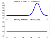
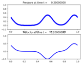
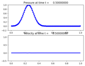
Here p is the pressure, u is the velocity, K is the bulk modulus, and \(\rho\) is the density.

The initial condition is a Gaussian and the boundary conditions are periodic. The final solution is identical to the initial data because both waves have crossed the domain exactly once.

Output:

Source:

#!/usr/bin/env python
# encoding: utf-8

r"""
One-dimensional acoustics
=========================

Solve the (linear) acoustics equations:

.. math::
    p_t + K u_x & = 0 \\
    u_t + p_x / \rho & = 0.

Here p is the pressure, u is the velocity, K is the bulk modulus,
and :math:`\rho` is the density.

The initial condition is a Gaussian and the boundary conditions are periodic.
The final solution is identical to the initial data because both waves have
crossed the domain exactly once.
"""
from numpy import sqrt, exp, cos
from clawpack import riemann


def setup(use_petsc=False, kernel_language='Fortran', solver_type='classic',
          outdir='./_output', ptwise=False, weno_order=5,
          time_integrator='SSP104', disable_output=False, output_style=1):

    if use_petsc:
        import clawpack.petclaw as pyclaw
    else:
        from clawpack import pyclaw

    if kernel_language == 'Fortran':
        if ptwise:
            riemann_solver = riemann.acoustics_1D_ptwise
        else:
            riemann_solver = riemann.acoustics_1D

    elif kernel_language == 'Python':
        riemann_solver = riemann.acoustics_1D_py.acoustics_1D

    if solver_type == 'classic':
        solver = pyclaw.ClawSolver1D(riemann_solver)
        solver.limiters = pyclaw.limiters.tvd.MC
    elif solver_type == 'sharpclaw':
        solver = pyclaw.SharpClawSolver1D(riemann_solver)
        solver.weno_order = weno_order
        solver.time_integrator = time_integrator
        if time_integrator == 'SSPLMMk3':
            solver.lmm_steps = 4
    else:
        raise Exception('Unrecognized value of solver_type.')

    solver.kernel_language = kernel_language

    x = pyclaw.Dimension(0.0, 1.0, 100, name='x')
    domain = pyclaw.Domain(x)
    num_eqn = 2
    state = pyclaw.State(domain, num_eqn)

    solver.bc_lower[0] = pyclaw.BC.periodic
    solver.bc_upper[0] = pyclaw.BC.periodic

    rho = 1.0   # Material density
    bulk = 1.0  # Material bulk modulus

    state.problem_data['rho'] = rho
    state.problem_data['bulk'] = bulk
    state.problem_data['zz'] = sqrt(rho*bulk)   # Impedance
    state.problem_data['cc'] = sqrt(bulk/rho)   # Sound speed

    xc = domain.grid.x.centers
    beta = 100
    gamma = 0
    x0 = 0.75
    state.q[0, :] = exp(-beta * (xc-x0)**2) * cos(gamma * (xc - x0))
    state.q[1, :] = 0.0

    solver.dt_initial = domain.grid.delta[0] / state.problem_data['cc'] * 0.1

    claw = pyclaw.Controller()
    claw.solution = pyclaw.Solution(state, domain)
    claw.solver = solver
    claw.outdir = outdir
    claw.output_style = output_style
    if output_style == 1:
        claw.tfinal = 1.0
        claw.num_output_times = 10
    elif output_style == 3:
        claw.nstep = 1
        claw.num_output_times = 1
    claw.keep_copy = True
    if disable_output:
        claw.output_format = None
    claw.setplot = setplot

    return claw


def setplot(plotdata):
    """
    Specify what is to be plotted at each frame.
    Input:  plotdata, an instance of visclaw.data.ClawPlotData.
    Output: a modified version of plotdata.
    """
    plotdata.clearfigures()  # clear any old figures,axes,items data

    # Figure for pressure
    plotfigure = plotdata.new_plotfigure(name='Pressure', figno=1)

    # Set up for axes in this figure:
    plotaxes = plotfigure.new_plotaxes()
    plotaxes.axescmd = 'subplot(211)'
    plotaxes.ylimits = [-0.2, 1.0]
    plotaxes.title = 'Pressure'

    # Set up for item on these axes:
    plotitem = plotaxes.new_plotitem(plot_type='1d_plot')
    plotitem.plot_var = 0
    plotitem.plotstyle = '-o'
    plotitem.color = 'b'
    plotitem.kwargs = {'linewidth': 2, 'markersize': 5}

    # Set up for axes in this figure:
    plotaxes = plotfigure.new_plotaxes()
    plotaxes.axescmd = 'subplot(212)'
    plotaxes.xlimits = 'auto'
    plotaxes.ylimits = [-0.5, 1.1]
    plotaxes.title = 'Velocity'

    # Set up for item on these axes:
    plotitem = plotaxes.new_plotitem(plot_type='1d_plot')
    plotitem.plot_var = 1
    plotitem.plotstyle = '-'
    plotitem.color = 'b'
    plotitem.kwargs = {'linewidth': 3, 'markersize': 5}

    return plotdata


def run_and_plot(**kwargs):
    claw = setup(kwargs)
    claw.run()
    from clawpack.pyclaw import plot
    plot.interactive_plot(setplot=setplot)

if __name__ == "__main__":
    from clawpack.pyclaw.util import run_app_from_main
    output = run_app_from_main(setup, setplot)