2-dimensional Euler equations

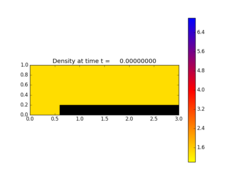
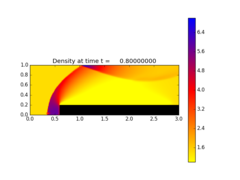
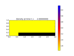
Compressible Euler flow over a forward-facing step

Solve the Euler equations of compressible fluid dynamics in 2D:

\[\begin{split}\rho_t + (\rho u)_x + (\rho v)_y = 0 \\ (\rho u)_t + (\rho u^2 + p)_x + (\rho uv)_y = 0 \\ (\rho v)_t + (\rho uv)_x + (\rho v^2 + p)_y = 0 \\ E_t + (u (E + p) )_x + (v (E + p))_y = 0.\end{split}\]

Here \(\rho\) is the density, (u,v) is the velocity, and E is the total energy.

The problem involves a shock wave impacting a forward-facing step. A stationary shock forms. When using a Roe solver, there is a carbuncle instability.

This example demonstrates how to include internal boundaries within the domain. An aux array field is used to indicate which cells are inside (1) or outside (0) of the domain. A special Riemann solver enforces reflecting boundary conditions at the internal boundaries. This could be modified to handle other internal boundary geometries, as long as they are aligned with the grid.

Output:

Source:

#!/usr/bin/env python
# encoding: utf-8
r"""
Compressible Euler flow over a forward-facing step
==================================================

Solve the Euler equations of compressible fluid dynamics in 2D:

.. math::
    \rho_t + (\rho u)_x + (\rho v)_y = 0 \\
    (\rho u)_t + (\rho u^2 + p)_x + (\rho uv)_y = 0 \\
    (\rho v)_t + (\rho uv)_x + (\rho v^2 + p)_y = 0 \\
    E_t + (u (E + p) )_x + (v (E + p))_y = 0.


Here :math:`\rho` is the density, (u,v) is the velocity, and E is the total energy.

The problem involves a shock wave impacting a forward-facing step.  A
stationary shock forms.  When using a Roe solver, there is a carbuncle
instability.

This example demonstrates how to include internal boundaries within the
domain.  An aux array field is used to indicate which cells are inside (1)
or outside (0) of the domain.  A special Riemann solver enforces reflecting
boundary conditions at the internal boundaries.  This could be modified
to handle other internal boundary geometries, as long as they are
aligned with the grid.
"""

from __future__ import absolute_import
from six.moves import range

gamma = 1.4 # Ratio of specific heats

def incoming_shock(state,dim,t,qbc,auxbc,num_ghost):
    """
    Incoming shock at left boundary.
    """
    rho = 1.4
    u   = 3.0
    v   = 0.0
    p   = 1.0
    T   = 2*p/rho

    for i in range(num_ghost):
        qbc[0,i,...] = rho
        qbc[1,i,...] = rho*u
        qbc[2,i,...] = rho*v
        qbc[3,i,...] = rho*(5.0/4 * T + (u**2+v**2)/2.)


def setup(use_petsc=False,solver_type='classic', outdir='_output', kernel_language='Fortran',
          disable_output=False, mx=320, my=80, tfinal=2.0, num_output_times = 10):

    if use_petsc:
        import clawpack.petclaw as pyclaw
    else:
        from clawpack import pyclaw

    from clawpack import riemann

    if solver_type=='sharpclaw':
        #solver = pyclaw.SharpClawSolver2D(euler_with_boundaries)
        raise Exception('This problem does not currently work with SharpClaw')
    else:
        solver = pyclaw.ClawSolver2D(riemann.euler_hlle_with_walls_2D)
        solver.dimensional_split = True

    solver.num_eqn = 4
    solver.num_waves = 4
    num_aux = 1

    x = pyclaw.Dimension(0.0,3.0,mx,name='x')
    y = pyclaw.Dimension(0.0,1.0,my,name='y')
    domain = pyclaw.Domain([x,y])

    state = pyclaw.State(domain,solver.num_eqn,num_aux)
    state.problem_data['gamma']= gamma

    solver.user_bc_lower = incoming_shock

    solver.bc_lower[0]=pyclaw.BC.custom
    solver.bc_upper[0]=pyclaw.BC.extrap
    solver.bc_lower[1]=pyclaw.BC.wall
    solver.bc_upper[1]=pyclaw.BC.wall

    solver.aux_bc_lower[0]=pyclaw.BC.extrap
    solver.aux_bc_upper[0]=pyclaw.BC.extrap
    solver.aux_bc_lower[1]=pyclaw.BC.wall
    solver.aux_bc_upper[1]=pyclaw.BC.wall

    rho = 1.4
    u = 3.0
    v = 0.
    p = 1.0
    T = 2*p/rho

    state.q[0,...] = rho
    state.q[1,...] = rho*u
    state.q[2,...] = rho*v
    state.q[3,...] = rho*(5.0/4 * T + (u**2+v**2)/2.)

    x,y = domain.grid.p_centers

    # Set aux values to zero inside step, to unity elsewhere
    state.aux[0,...]= 1 - (x > 0.6)*(y < 0.2)

    claw = pyclaw.Controller()
    claw.solution = pyclaw.Solution(state,domain)
    claw.solver = solver

    claw.keep_copy = True
    if disable_output:
        claw.output_format = None
    claw.tfinal = tfinal
    claw.num_output_times = num_output_times
    claw.outdir = outdir
    claw.setplot = setplot

    return claw

    
def setplot(plotdata):
    "Plot solution using VisClaw." 
    from clawpack.visclaw import colormaps

    plotdata.clearfigures()  # clear any old figures,axes,items data
    
    # Density plot
    plotfigure = plotdata.new_plotfigure(name='Density', figno=0)

    plotaxes = plotfigure.new_plotaxes()
    plotaxes.title = 'Density'
    plotaxes.scaled = True      # so aspect ratio is 1
    plotaxes.afteraxes = fill_step
    plotitem = plotaxes.new_plotitem(plot_type='2d_pcolor')
    plotitem.plot_var = 0
    plotitem.pcolor_cmin = 1
    plotitem.pcolor_cmax = 7.0
    plotitem.add_colorbar = True
    

    # Schlieren plot of density
    plotfigure = plotdata.new_plotfigure(name='Schlieren', figno=1)

    plotaxes = plotfigure.new_plotaxes()
    plotaxes.title = 'Density (Schlieren)'
    plotaxes.scaled = True      # so aspect ratio is 1
    
    plotaxes.afteraxes = fill_step
    plotitem = plotaxes.new_plotitem(plot_type='2d_schlieren')
    plotitem.schlieren_cmin = 0.
    plotitem.schlieren_cmax = 3.
    plotitem.plot_var = 0
    plotitem.add_colorbar = False
    
    return plotdata
   
def fill_step(_):
    "Fill the step area with a black rectangle."
    import matplotlib.pyplot as plt
    rectangle = plt.Rectangle((0.6,0.0),2.4,0.2,color="k",fill=True)
    plt.gca().add_patch(rectangle)


if __name__=="__main__":
    from clawpack.pyclaw.util import run_app_from_main
    output = run_app_from_main(setup,setplot)