1-dimensional Euler equations

Woodward-Colella blast wave problem

Solve the one-dimensional Euler equations for inviscid, compressible flow:

\[\begin{split}\rho_t + (\rho u)_x & = 0 \\ (\rho u)_t + (\rho u^2 + p)_x & = 0 \\ E_t + (u (E + p) )_x & = 0.\end{split}\]

The fluid is an ideal gas, with pressure given by \(p=\rho (\gamma-1)e\) where e is internal energy.

This script runs the Woodward-Colella blast wave interaction problem, involving the collision of two shock waves.

This example also demonstrates:

• How to use a total fluctuation solver in SharpClaw

• How to use characteristic decomposition with an evec() routine in SharpClaw

Output:

Source:

#!/usr/bin/env python
# encoding: utf-8
r"""
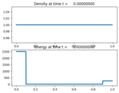
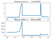
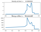
Woodward-Colella blast wave problem
===================================

Solve the one-dimensional Euler equations for inviscid, compressible flow:

.. math::
    \rho_t + (\rho u)_x & = 0 \\
    (\rho u)_t + (\rho u^2 + p)_x & = 0 \\
    E_t + (u (E + p) )_x & = 0.

The fluid is an ideal gas, with pressure given by :math:`p=\rho (\gamma-1)e` where
e is internal energy.

This script runs the Woodward-Colella blast wave interaction problem,
involving the collision of two shock waves.

This example also demonstrates:

 - How to use a total fluctuation solver in SharpClaw
 - How to use characteristic decomposition with an evec() routine in SharpClaw
"""
from clawpack import riemann
from clawpack.riemann.euler_with_efix_1D_constants import *

gamma = 1.4 # Ratio of specific heats

def setup(use_petsc=False,outdir='./_output',solver_type='sharpclaw',kernel_language='Fortran',tfluct_solver=True):

    if use_petsc:
        import clawpack.petclaw as pyclaw
    else:
        from clawpack import pyclaw

    if kernel_language =='Python':
        rs = riemann.euler_1D_py.euler_roe_1D
    elif kernel_language =='Fortran':
        rs = riemann.euler_with_efix_1D

    if solver_type=='sharpclaw':
        solver = pyclaw.SharpClawSolver1D(rs)
        solver.time_integrator = 'SSP33'
        solver.cfl_max = 0.65
        solver.cfl_desired = 0.6
        solver.tfluct_solver = tfluct_solver
        if solver.tfluct_solver:
            from clawpack.pyclaw.sharpclaw import euler_tfluct1
            solver.tfluct = euler_tfluct1
        solver.lim_type = 1
        solver.char_decomp = 2
        from clawpack.pyclaw.sharpclaw import euler_sharpclaw1
        solver.fmod = euler_sharpclaw1
    elif solver_type=='classic':
        solver = pyclaw.ClawSolver1D(rs)
        solver.limiters = 4

    solver.kernel_language = kernel_language

    solver.bc_lower[0]=pyclaw.BC.wall
    solver.bc_upper[0]=pyclaw.BC.wall

    mx = 800;
    x = pyclaw.Dimension(0.0,1.0,mx,name='x')
    domain = pyclaw.Domain([x])
    state = pyclaw.State(domain,num_eqn)

    state.problem_data['gamma'] = gamma
    if kernel_language =='Python':
        state.problem_data['efix'] = False

    x = state.grid.x.centers

    state.q[density ,:] = 1.
    state.q[momentum,:] = 0.
    state.q[energy  ,:] = ( (x<0.1)*1.e3 + (0.1<=x)*(x<0.9)*1.e-2 + (0.9<=x)*1.e2 ) / (gamma - 1.)

    claw = pyclaw.Controller()
    claw.tfinal = 0.038
    claw.solution = pyclaw.Solution(state,domain)
    claw.solver = solver
    claw.num_output_times = 10
    claw.outdir = outdir
    claw.setplot = setplot
    claw.keep_copy = True

    return claw

#--------------------------
def setplot(plotdata):
#--------------------------
    """ 
    Specify what is to be plotted at each frame.
    Input:  plotdata, an instance of visclaw.data.ClawPlotData.
    Output: a modified version of plotdata.
    """ 
    plotdata.clearfigures()  # clear any old figures,axes,items data

    plotfigure = plotdata.new_plotfigure(name='', figno=0)

    plotaxes = plotfigure.new_plotaxes()
    plotaxes.axescmd = 'subplot(211)'
    plotaxes.title = 'Density'

    plotitem = plotaxes.new_plotitem(plot_type='1d')
    plotitem.plot_var = density
    plotitem.kwargs = {'linewidth':3}
    
    plotaxes = plotfigure.new_plotaxes()
    plotaxes.axescmd = 'subplot(212)'
    plotaxes.title = 'Energy'

    plotitem = plotaxes.new_plotitem(plot_type='1d')
    plotitem.plot_var = energy
    plotitem.kwargs = {'linewidth':3}
    
    return plotdata

if __name__=="__main__":
    from clawpack.pyclaw.util import run_app_from_main
    output = run_app_from_main(setup,setplot)