Nonlinear elasticity
%matplotlib inline
%config InlineBackend.figure_format = 'svg'
import matplotlib as mpl
mpl.rcParams['font.size'] = 8
figsize =(8,4)
mpl.rcParams['figure.figsize'] = figsize

import numpy as np
from scipy.optimize import fsolve
import matplotlib.pyplot as plt
from utils import riemann_tools
from utils.snapshot_widgets import interact
from ipywidgets import widgets
from clawpack import riemann
from exact_solvers import nonlinear_elasticity
In this chapter we investigate a nonlinear model of elastic strain in heterogeneous materials. This system is equivalent to the $p$-system of gas dynamics, although the stress-strain relation we will use here is very different from the pressure-density relation typically used in gas dynamics. The equations we consider are:
\begin{align} \epsilon_t(x,t) - u_x(x,t) & = 0 \\ (\rho(x)u(x,t))_t - \sigma(\epsilon(x,t),x)_x & = 0. \end{align}
Here $\epsilon$ is the strain, $u$ is the velocity, $\rho$ is the material density, $\sigma$ is the stress, and ${\mathcal M}=\rho u$ is the momentum. The first equation is a kinematic relation, while the second represents Newton's second law. This is a nonlinear conservation law with spatially varying flux function, in which
\begin{align} q & = \begin{bmatrix} \epsilon \\ \rho u \end{bmatrix}, & f(q,x) & = \begin{bmatrix} -{\mathcal M}/\rho(x) \\ -\sigma(\epsilon,x) \end{bmatrix}. \end{align}
If the stress-strain relationship is linear -- i.e. if $\sigma(\epsilon,x)=K(x)\epsilon$ -- then this system is equivalent to the acoustics equations that we have studied previously. Here we consider instead a quadratic stress response:
\begin{align} \sigma(\epsilon,x) = K_1(x) \epsilon + K_2(x) \epsilon^2. \end{align}
We assume that the spatially-varying functions $\rho, K_1, K_2$ are piecewise constant, taking values $(\rho_l, K_{1l}, K_{2l})$ for $x<0$ and values $(\rho_r, K_{1r}, K_{2r})$ for $x>0$. This system has been investigated numerically in (LeVeque, 2002), (LeVeque & Yong, 2003), and (Ketcheson & LeVeque, 2012).
Note that if we take $\rho=1$, $\sigma=-p$, and $\epsilon=v$, this system is equivalent to the p-system of Lagrangian gas dynamics \begin{align*} v_t - u_x & = 0 \\ u_t - p(v)_x & = 0, \end{align*} in which $p$ represents pressure and $v$ represents specific volume.
Hyperbolic structure
The flux jacobian is
\begin{align} f'(q) = \begin{bmatrix} 0 & -1/\rho(x) \\ -\sigma_\epsilon(\epsilon,x) & 0 \end{bmatrix}, \end{align}
with eigenvalues (characteristic speeds)
\begin{align} \lambda^\pm(x) = \pm \sqrt{\frac{\sigma_\epsilon(\epsilon,x)}{\rho(x)}} = \pm c(\epsilon, x). \end{align}
Here for the stress-strain relation we have chosen, $\sigma_\epsilon = K_1(x) + 2 K_2(x)\epsilon$.
It's also convenient to define the nonlinear impedance $Z(\epsilon, x) = \rho(x) c(\epsilon,x)$. Then the eigenvectors of the flux Jacobian are
\begin{align} R & = \begin{bmatrix} 1 & 1 \\ Z(\epsilon,x) & -Z(\epsilon,x) \end{bmatrix}. \end{align}
Both characteristic fields are genuinely nonlinear. Furthermore, since the characteristic speeds each have a definite sign, this system does not admit transonic rarefactions.
Structure of the Riemann solution
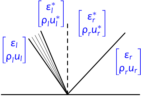
Based on the eigenstructure of the flux jacobian above, the Riemann solution will always include a left-going and a right-going wave, each of which may be a shock or rarefaction (since both fields are genuinely nonlinear). We will see -- similarly to our analysis in the chapter on variable-speed-limit traffic that the jump in $\rho$ and $K$ at $x=0$ induces a stationary wave there. See the figure below for the overall structure of the Riemann solution.
Hugoniot loci
From the Rankine-Hugoniot jump conditions for the system we obtain the 1-Hugoniot locus for a state $(\epsilon^*_l, u^*_l)$ connected by a 1-shock to a state $(\epsilon_l, u_l)$:
\begin{align} u^*_l & = u_l - \left( \frac{\left(\sigma_l(\epsilon^*_l)-\sigma_l(\epsilon_l)\right)(\epsilon^*_l-\epsilon_l)}{\rho_l} \right)^{1/2} \end{align}
Here $\sigma_l(\epsilon)$ is shorthand for the stress relation in the left medium. Similarly, a state $(\epsilon^*_r,u^*_r)$ that is connected by a 2-shock to a state $(\epsilon_r, u_r)$ must satisfy
\begin{align} u^*_r & = u_r - \left( \frac{\left(\sigma_r(\epsilon^*_r)-\sigma_r(\epsilon_r)\right)(\epsilon^*_r-\epsilon_r)}{\rho_r} \right)^{1/2}. \end{align}
Integral curves
The integral curves can be found by writing $\tilde{q}'(\xi) = r^{1,2}(\tilde{q}(\xi))$ and integrating. This leads to \begin{align} u^*_l & = u_l + \frac{1}{3 K_{2l} \sqrt{\rho_l}} \left( \sigma_{l,\epsilon}(\epsilon^*_l)^{3/2} - \sigma_{l,\epsilon}(\epsilon)^{3/2} \right) \label{NE:integral-curve-1} \\ u^*_r & = u_r - \frac{1}{3 K_{2r} \sqrt{\rho_r}} \left( \sigma_{r,\epsilon}(\epsilon^*_r)^{3/2} - \sigma_{r,\epsilon}(\epsilon)^{3/2} \right)\label{NE:integral-curve-2} \end{align} Here $\sigma_{l,\epsilon}$ is the derivative of the stress function w.r.t $\epsilon$ in the left medium.
The entropy condition
For a 1-shock, we need that $\lambda^-(\epsilon_l,x<0) > \lambda^-(\epsilon^*_l,x<0)$, which is equivalent to the condition $\epsilon^*_l>\epsilon_l$. Similarly, a 2-shock is entropy-satisfying if $\epsilon^*_r > \epsilon_r$.
Interface conditions
Because the flux depends explicitly on $x$, we do not necessarily have continuity of $q$ at $x=0$; i.e. in general $q^*_l \ne q^*_r$. Instead, the flux must be continuous: $f(q^*_l)=f(q^*_r)$. For the present system, this means that the stress and velocity must be continuous:
\begin{align*} u^*_l & = u^*_r \\ \sigma(\epsilon^*_l, K_{1l}, K_{2l}) & = \sigma(\epsilon^*_r, K_{1r}, K_{2r}). \end{align*}
This makes sense from a physical point of view: if the velocity were not continuous, the material would fracture (or overlap itself). Continuity of the stress is required by Newton's laws.
Structure of rarefaction waves
For this system, the structure of a centered rarefaction wave can be determined very simply. Since the characteristic velocity must be equal to $\xi = x/t$ at each point along the wave, we have $\xi = \pm\sqrt{\sigma_\epsilon/\rho}$, or \begin{align} \xi^2 = \frac{K_1 + 2K_2\epsilon}{\rho} \end{align} which leads to $\epsilon = (\rho\xi^2 - K_1)/(2K_2)$. Once the value of $\epsilon$ is known, $u$ can be determined using the integral curves \eqref{NE:integral-curve-1} or \eqref{NE:integral-curve-2}.
Solution of the Riemann problem
Below we show the solution of the Riemann problem. To view the code that computes this exact solution, uncomment and execute the next cell.
# %load exact_solvers/nonlinear_elasticity.py
def dsigma(eps, K1, K2):
    "Derivative of stress w.r.t. strain."
    return K1 + 2*K2*eps

def lambda1(q, xi, aux):
    eps = q[0]
    rho, K1, K2 = aux
    return -np.sqrt(dsigma(eps, K1, K2)/rho)

def lambda2(q, xi, aux):
    return -lambda1(q,xi,aux)
def make_plot_function(q_l, q_r, aux_l, aux_r):
    states, speeds, reval, wave_types = \
        nonlinear_elasticity.exact_riemann_solution(q_l,q_r,aux_l,aux_r)

    def plot_function(t,which_char):
        ax = riemann_tools.plot_riemann(states,speeds,reval,wave_types,
                                        t=t,t_pointer=0,
                                        extra_axes=True,
                                        variable_names=['Strain','Momentum'])
        if which_char == 1:
            riemann_tools.plot_characteristics(reval,lambda1,(aux_l,aux_r),ax[0])
        elif which_char == 2:
            riemann_tools.plot_characteristics(reval,lambda2,(aux_l,aux_r),ax[0])
        nonlinear_elasticity.phase_plane_plot(q_l, q_r, aux_l, aux_r, ax[3])
        plt.show()
    return plot_function

def plot_riemann_nonlinear_elasticity(rho_l,rho_r,v_l,v_r):
    plot_function = make_plot_function(rho_l,rho_r,v_l,v_r)
    interact(plot_function, t=widgets.FloatSlider(value=0.,min=0,max=1.,step=0.1),
             which_char=widgets.Dropdown(options=[None,1,2],
                                         description='Show characteristics'));
aux_l = np.array((1., 5., 1.))
aux_r = np.array((1., 2., 1.))
q_l = np.array([2.1, 0.])
q_r = np.array([0.0, 0.])

plot_riemann_nonlinear_elasticity(q_l, q_r, aux_l, aux_r)
Approximate solution of the Riemann problem using $f$-waves
The exact solver above requires a nonlinear iterative rootfinder and is relatively expensive. A very cheap approximate Riemann solver for this system was developed in (LeVeque, 2002) using the $f$-wave approach. One simply approximates both nonlinear waves as shocks, with speeds equal to the characteristic speeds of the left and right states:
\begin{align} s^1 & = - \sqrt{\frac{\sigma_{\epsilon,l}(\epsilon_l)}{\rho_l}} \\ s^2 & = + \sqrt{\frac{\sigma_{\epsilon,r}(\epsilon_r)}{\rho_r}}. \end{align}
Meanwhile, the waves are obtained by decomposing the jump in the flux $f(q_r,x>0) - f(q_l,x<0)$ in terms of the eigenvectors of the flux jacobian.
solver = riemann.nonlinear_elasticity_1D_py.nonlinear_elasticity_1D

problem_data = {'stress_relation' : 'quadratic'}
fw_states, fw_speeds, fw_reval = \
            riemann_tools.riemann_solution(solver,q_l,q_r,aux_l,aux_r,
                                           problem_data=problem_data,
                                           verbose=False,
                                           stationary_wave=True,
                                           fwave=True)
plot_function = \
    riemann_tools.make_plot_function(fw_states,fw_speeds, fw_reval,
                                     layout='vertical',
                                     variable_names=('Strain','Momentum'))
interact(plot_function, t=widgets.FloatSlider(value=0.4,min=0,max=.9,step=.1));
Comparison of exact and approximate solutions
ex_states, ex_speeds, ex_reval, wave_types = \
            nonlinear_elasticity.exact_riemann_solution(q_l,q_r,aux_l,aux_r)

varnames = nonlinear_elasticity.conserved_variables
plot_function = riemann_tools.make_plot_function([ex_states,fw_states],
                                                 [ex_speeds,fw_speeds],
                                                 [ex_reval,fw_reval],
                                                 [wave_types,['contact']*3],
                                                 ['Exact','$f$-wave'],
                                                 layout='vertical',
                                                 variable_names=varnames)
interact(plot_function, t=widgets.FloatSlider(value=0.4,min=0, max=0.9, step=0.1));
As we can see, there are significant discrepancies between the approximate solution and the exact one. But in a full numerical discretization, the left- and right-going waves are averaged over neighboring cells at the next step, and the approximate solver yields an effective result quite close to that of the exact solver.