Wave tank simulation compared to USACE experiment

This example is based on a wave tank experiment that was performed by the US Army Corps of Engineers (USACE) and has been used as a test problem in several papers, in particular in

Synolakis, C.E., E.N. Bernard, V.V. Titov, U. Kânoğlu, and F.I. González (2007): Standards, criteria, and procedures for NOAA evaluation of tsunami numerical models. NOAA Tech. Memo. OAR PMEL-135, NOAA/Pacific Marine Environmental Laboratory, Seattle, WA https://nctr.pmel.noaa.gov/benchmark/

The problem is described at https://nctr.pmel.noaa.gov/benchmark/Solitary_wave/

The file tsunami3_runup.zip containing observations from the experiment was obtained from that webpage and unzipped to obtain data in directory experimental_data.

qinit.f90 is set up for case B with amplitude H/d = 0.259.

The file make_celledges.py sets up the domain and computational grid. A piecewise linear topography is defined by specifying the topography z value at a set of nodes x in the xzpairs list. The topography is based on the Revere Beach composite beach geometry used in the physical wave tank.

A nonuniform grid with mx grid cells is used with cell widths related to the still water depth in such a way that the Courant number is roughly constant in deep water and onto the shelf, and with uniform grid cells near shore and onshore where the water depth is less than hmin.

Executing make_celledges.py creates a file celledges.data that contains the cell edges. This file must be created before running GeoClaw.

In GeoClaw a mapped grid is used with a mapc2p function specified in setrun.py that is generated from the celledges.data. The computational grid specified in setrun.py is always 0 <= xc <= 1. Set:

rundata.grid_data.grid_type = 2

to indicate a mapped grid.

In this example the physical x coordiate is in meters, set by specifying:

rundata.geo_data.coordinate_system = 1

To use:

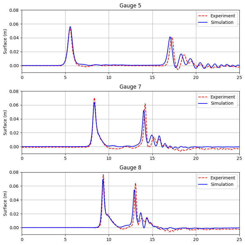
make topo     # executes make_celledges.py
make .output  # compile, make data, and run
make .plots   # to create _plots (or plot interactively with Iplotclaw)

python compare_gauges.py  # to create a plot of gauges to compare to paper

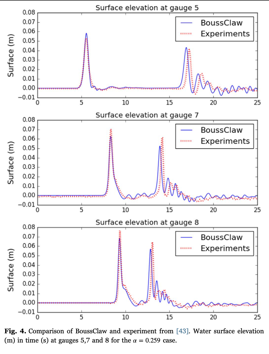
The figure generated should be similar to GeoClawGaugeComparison.png, and can be compared to KimFigure4.png, which is Figure 4 in the original BoussClaw paper

Kim, J., Pedersen, G. K., Løvholt, F. & LeVeque, R. J., A Boussinesq type extension of the GeoClaw model - a study of wave breaking phenomena applying dispersive long wave models. Coastal Engineering 122, 75–86 (2017). http://dx.doi.org/10.1016/j.coastaleng.2017.01.005

This plot shows the time history at gauges 5, 7, and 8. See that paper for additional details on the problem and data.

See also compare_BoussSWE.py, which runs the code with various settings and plots the results together. This file could be modified to perform additional tests, but as provided it runs the SGN model with alpha=1.153, the MS model with B=1/15, and the non-dispersive shallow water equations. This should produce a figure similar to GeoClawGaugeComparison_BoussSWE.png,