
This example illustrates the use of an fgmax grid and an fgout grid, which can be used independently of one another.
For details about this test problem, see $CLAW/geoclaw/examples/tsunami/chile2010.
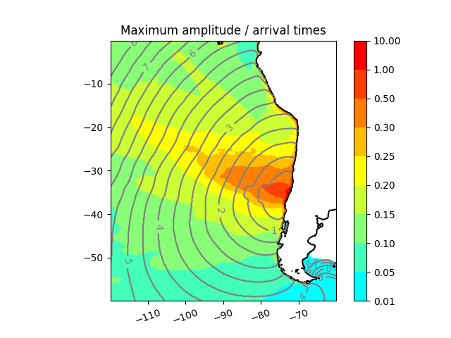
See https://www.clawpack.org/fgmax.html for general documentation of fgmax grids. In this example, an fgmax grid is used to monitor the maximum amplitude of the wave at each point in the domain and the arrival times, in order to make a plot displaying these over the computational domain, a portion of the south Pacific.
The fgmax grid is specified in setrun.py and doing make data (or make .output) leads to the creation of a file fgmax_grids.data that is read into GeoClaw.
To test:
make topo
make .output
make plots             # to make frame plots and _PlotIndex.html
Or simply:
make all
This should produce _plots/amplitude_times.png, a color map of maximum amplitudes along with contours of arrival time. This is generated by the code in plot_fgmax.py and a link to this plot should show up in _plots/_PlotIndex.html along with the usual time frame plots.
Note:
See http://www.clawpack.org/fgmax.html for more information about specifying fgmax parameters.
The time fg.tstart_max in setrun.py is set to 10 seconds so that the topography in the source region has been finalized following the earthquake before we start monitoring the maxima. (Since the topo on the fixed grid must also be stored for later postprocessing.)
The refinement parameters and regions are set so that the maximum amplitude we wish to capture always appears on a level 3 grid and fg.min_level_check = 3 is set in setrun.py. Other choices of these parameters may give misleading or bizarre results. The fgmax capabilities were designed with the assumption that the region of interest will always be refined to the maximum level allowed.
The code in plot_fgmax.py is used to plot the fgmax results. Also the file setplot.py includes the lines:
otherfigure = plotdata.new_otherfigure(name='max amplitude and arrival times',
             fname='amplitude_times.png')

 def makefig(plotdata):
     plot_fgmax.plot_fgmax_grid(plotdata.outdir, plotdata.plotdir)

 otherfigure.makefig = makefig
This results in plot_fgmax.plot_fgmax_grid being run and the link to the resulting figure appearing in _plots/_PlotIndex.html.
See https://www.clawpack.org/fgout.html for general documentation of fgout grids. Here a single fgout grid is specified in setrun.py that covers most of the computational domain at a fixed resolution. The solution interpolated to this grid is output every 15 minutes, more frequently than the usual GeoClaw frames, which in this example are output only every 2 hours.
To test:
make all
as suggested above also makes _plots_fgout with illustrations of fgout plots and animations.
This does the following, which you can also do directly at the command line:
make plots SETPLOT_FILE=setplot_fgout.py PLOTDIR=_plots_fgout
This illustrates one approach to plotting fgout grid results: A setplot function is specified (in this case by setplot_fgout.py) that has the same form as a setplot function for plotting standard GeoClaw/Clawpack output frames, but in setplot_fgout.py we set
plotdata.file_prefix = 'fgout0001' # for fgout grid fgno==1
to indicate that instead of the usual output files with names like fort.t* and fort.q* (and also fort.b* in the case of binary output), as described at https://www.clawpack.org/output_styles.html, the data is in files named fgout0001.t*, etc. but with the same format.
This creates the usual sort of _plots directory displaying all the resulting fgout plots. In this example we have called this directory _plots_fgout to differentiate it from the directory _plots which contains the usual plots from output times.
Alternatively, since every fgout frame consists of only a single uniform grid of data, it is much easier to manipulate or plot directly than general AMR data. The clawpack.geoclaw.fgout_tools module described at https://www.clawpack.org/fgout_tools_module.html provides tools for reading frames and producing arrays that can then be worked with directly.
An example of how this might be done is provided in plot_fgout.py, where a single frame is plotted. To test this do:
python plot_fgout.py
and a single png file will be created.
The sample code in make_fgout_animation.py reads in all the frames of fgout data and produces an animation as stand-alone mp4 and/or html files. To run this code, do:
python make_fgout_animation.py
Note that this is done automatically by make fgout_plots (which in turn is done automatically by make all), in which case the resulting animations fgout_animation.mp4 and fgout_animation.html are also moved into _plots_fgout.
The use of fgout grids provides a way to produce frequent outputs on a fixed grid resolution, as often desired for making smooth animations of a portion of the computational domain.
The script make_netcdf.py illustrates how to combine multiple fgout frames of data into a single netCDF file using fgout_tools.write_netcdf. This is easily done since all the fgout results are on the same uniform grid. You can also select which quantities of interest to store and use 32-bit floats to store them.
The script make_netcdf.py also illustrates how to read the arrays back in from the netCDF file. Test it using:
python make_netcdf.py
This example requires the Python module netCDF4.