2-dimensional variable-coefficient acoustics

Output:

Source:

#!/usr/bin/env python
# encoding: utf-8
r"""
Two-dimensional variable-coefficient acoustics on a mapped grid
===============================================================

Solve the variable-coefficient acoustics equations in 2D:

.. math:: 
    p_t + K(x,y) (u_x + v_y) & = 0 \\ 
    u_t + p_x / \rho(x,y) & = 0 \\
    v_t + p_y / \rho(x,y) & = 0.

Here p is the pressure, (u,v) is the velocity, :math:`K(x,y)` is the bulk modulus,
and :math:`\rho(x,y)` is the density.

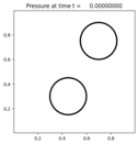
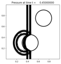
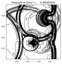
This example shows how to solve a problem with variable coefficients on a mapped grid.
The domain contains circular inclusions with different acoustic properties.
"""
import numpy as np

# Circle radius, square radius, circle center:
# ((r1, r2), (x0, y0))
circles = ( ((0.15,0.204),( 0.45,0.3)),
            ((0.15,0.204),( 0.7, 0.75)))

impedance = (12.,10.)
sound_speed = (0.3,1.5)

def inclusion_mapping(xc, yc):
    """Apply mapping from square to circle for each circle specified.
       Leave rest of grid cartesian.
    """
    xp = xc+0.
    yp = yc+0.

    for circle in circles:
        circle_center = circle[1]
        r1 = circle[0][0]
        r2 = circle[0][1]
    
        x0, y0 = circle_center
        xdist = np.abs(xc-x0)
        ydist = np.abs(yc-y0)
        insquare = np.where(np.maximum(xdist,ydist)<=r2) # Square section of grid to be deformed
        xc0 = (xc[insquare]-x0)/r2
        yc0 = (yc[insquare]-y0)/r2

        xc1 = np.abs(xc0)
        yc1 = np.abs(yc0)
        d = np.maximum(xc1, yc1)
        d = np.maximum(d,1.e-10)
        d = np.minimum(d, 0.99999)
        d1 = d*r2/np.sqrt(2)

        # Pick mapping
        #R = np.sqrt(2) * d1
        R = r1*np.ones(d1.shape)
        R = r1**2 / (r2*d)

        # Modify d1 and R outside circle to morph back to square:
        ij = np.where(d>(r1/r2))
        d1[ij] = r1/np.sqrt(2) + (d[ij]-r1/r2)*(r2-r1/np.sqrt(2))/(1.-r1/r2)
        R[ij] = r1 * ((1.-r1/r2) / (1.-d[ij]))**(r2/r1 + 0.5)

        xp2 = d1/d * xc1
        yp2 = d1/d * yc1
        center = d1 - np.sqrt(R**2 - d1**2)

        ij = np.where(xc1>=yc1)
        xp2[ij] = center[ij] + np.sqrt(R[ij]**2 - yp2[ij]**2)

        ij = np.where(yc1>=xc1)
        yp2[ij] = center[ij] + np.sqrt(R[ij]**2 - xp2[ij]**2)

        xp2 = np.sign(xc0) * xp2
        yp2 = np.sign(yc0) * yp2

        xp[insquare] = x0 + xp2
        yp[insquare] = y0 + yp2
    
    return xp, yp

def compute_geometry(grid):
    r"""Computes
        a_x
        a_y
        length_ratio_left
        b_x
        b_y
        length_ratio_bottom
        cell_area
    """

    dx, dy = grid.delta
    area_min = 1.e6
    area_max = 0.0

    x_corners, y_corners = grid.p_nodes

    lower_left_y, lower_left_x = y_corners[:-1,:-1], x_corners[:-1,:-1]
    upper_left_y, upper_left_x = y_corners[:-1,1: ], x_corners[:-1,1: ]
    lower_right_y, lower_right_x = y_corners[1:,:-1], x_corners[1:,:-1]
    upper_right_y, upper_right_x = y_corners[1:,1: ], x_corners[1:,1: ]

    a_x =   upper_left_y - lower_left_y  #upper left and lower left
    a_y = -(upper_left_x - lower_left_x)
    anorm = np.sqrt(a_x**2 + a_y**2)
    a_x, a_y = a_x/anorm, a_y/anorm
    length_ratio_left = anorm/dy

    b_x = -(lower_right_y - lower_left_y)  #lower right and lower left
    b_y =   lower_right_x - lower_left_x
    bnorm = np.sqrt(b_x**2 + b_y**2)
    b_x, b_y = b_x/bnorm, b_y/bnorm
    length_ratio_bottom = bnorm/dx

    area = 0*grid.c_centers[0]
    area += 0.5 * (lower_left_y+upper_left_y)*(upper_left_x-lower_left_x)
    area += 0.5 * (upper_left_y+upper_right_y)*(upper_right_x-upper_left_x)
    area += 0.5 * (upper_right_y+lower_right_y)*(lower_right_x-upper_right_x)
    area += 0.5 * (lower_right_y+lower_left_y)*(lower_left_x-lower_right_x)
    area = area/(dx*dy)
    area_min = min(area_min, np.min(area))
    area_max = max(area_max, np.max(area))

    return a_x, a_y, length_ratio_left, b_x, b_y, length_ratio_bottom, area

def incoming_square_wave(state,dim,t,qbc,auxbc,num_ghost):
    """
    Incoming square wave at left boundary.
    """
    if t<0.05:
        s = 1.0
    else:
        s = 0.0

    for i in range(num_ghost):
        reflect_ind = 2*num_ghost - i - 1
        alpha = auxbc[0,i,:]
        beta  = auxbc[1,i,:]
        u_normal = alpha*qbc[1,reflect_ind,:] + beta*qbc[2,reflect_ind,:]
        u_tangential = -beta*qbc[1,reflect_ind,:] + alpha*qbc[2,reflect_ind,:]
        u_normal = 2.0*s - u_normal
        qbc[0,i,:] = qbc[0,reflect_ind,:]
        qbc[1,i,:] = alpha*u_normal - beta*u_tangential
        qbc[2,i,:] = beta*u_normal + alpha*u_tangential


def setup(kernel_language='Fortran', use_petsc=False, outdir='./_output', 
          solver_type='classic', time_integrator='SSP104', lim_type=2, 
          num_output_times=20, disable_output=False, num_cells=200):
    from clawpack import riemann

    if use_petsc:
        import clawpack.petclaw as pyclaw
    else:
        from clawpack import pyclaw

    riemann_solver = riemann.acoustics_mapped_2D

    if solver_type=='classic':
        solver=pyclaw.ClawSolver2D(riemann_solver)
        solver.dimensional_split=False
        solver.limiters = pyclaw.limiters.tvd.MC
    elif solver_type=='sharpclaw':
        solver=pyclaw.SharpClawSolver2D(riemann_solver)
        solver.time_integrator=time_integrator

    solver.bc_lower[0]=pyclaw.BC.custom
    solver.user_bc_lower = incoming_square_wave
    solver.bc_upper[0]=pyclaw.BC.extrap
    solver.bc_lower[1]=pyclaw.BC.extrap
    solver.bc_upper[1]=pyclaw.BC.extrap

    solver.aux_bc_lower[0]=pyclaw.BC.extrap
    solver.aux_bc_upper[0]=pyclaw.BC.extrap
    solver.aux_bc_lower[1]=pyclaw.BC.extrap
    solver.aux_bc_upper[1]=pyclaw.BC.extrap

    x = pyclaw.Dimension(0.,1.0,num_cells,name='x')
    y = pyclaw.Dimension(0.,1.0,num_cells,name='y')
    domain = pyclaw.Domain([x,y])

    num_eqn = 3
    num_aux = 9 # geometry (7), impedance, sound speed
    state = pyclaw.State(domain,num_eqn,num_aux)
    state.grid.mapc2p = inclusion_mapping

    a_x, a_y, length_left, b_x, b_y, length_bottom, area = compute_geometry(state.grid)

    state.aux[0,:,:] = a_x
    state.aux[1,:,:] = a_y
    state.aux[2,:,:] = length_left
    state.aux[3,:,:] = b_x
    state.aux[4,:,:] = b_y
    state.aux[5,:,:] = length_bottom
    state.aux[6,:,:] = area
    state.index_capa = 6 # aux[6,:,:] holds the capacity function

    grid = state.grid
    xp, yp = grid.p_centers
    state.aux[7,:,:] = 1.0 # Impedance
    state.aux[8,:,:] = 1.0 # Sound speed

    for i, circle in enumerate(circles):
        # Set impedance and sound speed in each inclusion
        radius = circle[0][0]
        x0, y0 = circle[1]
        distance = np.sqrt( (xp-x0)**2 + (yp-y0)**2 )
        in_circle = np.where(distance <= radius)
        state.aux[7][in_circle] = impedance[i]
        state.aux[8][in_circle] = sound_speed[i]

    # Set initial condition
    state.q[0,:,:] = 0.
    state.q[1,:,:] = 0.
    state.q[2,:,:] = 0.

    claw = pyclaw.Controller()
    claw.keep_copy = True
    if disable_output:
        claw.output_format = None
    claw.solution = pyclaw.Solution(state,domain)
    claw.solver = solver
    claw.outdir = outdir
    claw.tfinal = 0.9
    claw.num_output_times = num_output_times
    claw.write_aux_init = True
    claw.setplot = setplot
    if use_petsc:
        claw.output_options = {'format':'binary'}

    return claw


def setplot(plotdata):
    """ 
    Plot solution using VisClaw.

    This example shows how to mark an internal boundary on a 2D plot.
    """ 

    from clawpack.visclaw import colormaps

    plotdata.clearfigures()  # clear any old figures,axes,items data
    plotdata.mapc2p = inclusion_mapping
    
    # Figure for pressure
    plotfigure = plotdata.new_plotfigure(name='Pressure', figno=0)

    # Set up for axes in this figure:
    plotaxes = plotfigure.new_plotaxes()
    plotaxes.title = 'Pressure'
    plotaxes.scaled = True      # so aspect ratio is 1
    plotaxes.afteraxes = plot_circles

    # Set up for item on these axes:
    plotitem = plotaxes.new_plotitem(plot_type='2d_contour')
    plotitem.contour_nlevels = 100
    plotitem.contour_min = -2.51
    plotitem.contour_max = 2.51
    plotitem.plot_var = 0
    
    # Figure for x-velocity plot
    plotfigure = plotdata.new_plotfigure(name='x-Velocity', figno=1)

    # Set up for axes in this figure:
    plotaxes = plotfigure.new_plotaxes()
    plotaxes.title = 'u'
    plotaxes.afteraxes = plot_circles

    plotitem = plotaxes.new_plotitem(plot_type='2d_pcolor')
    plotitem.plot_var = 1
    plotitem.pcolor_cmap = 'RdBu'
    plotitem.add_colorbar = True
    plotitem.pcolor_cmin = -1.0
    plotitem.pcolor_cmax=   1.0
    
    return plotdata

def plot_circles(current_data):
    import matplotlib.pyplot as plt
    ax = plt.gca()
    for circle in circles:
        x0, y0 = circle[1]
        radius = circle[0][0]
        circle1=plt.Circle((x0,y0),radius,color='k',fill=False,lw=3)
        ax.add_artist(circle1)


if __name__=="__main__":
    import sys
    from clawpack.pyclaw.util import run_app_from_main
    output = run_app_from_main(setup,setplot)