2-dimensional variable-coefficient acoustics

Two-dimensional variable-coefficient acoustics

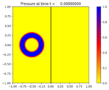
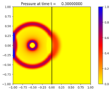
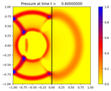
Solve the variable-coefficient acoustics equations in 2D:

\[\begin{split}p_t + K(x,y) (u_x + v_y) & = 0 \\ u_t + p_x / \rho(x,y) & = 0 \\ v_t + p_y / \rho(x,y) & = 0.\end{split}\]

Here p is the pressure, (u,v) is the velocity, \(K(x,y)\) is the bulk modulus, and \(\rho(x,y)\) is the density.

This example shows how to solve a problem with variable coefficients. The left and right halves of the domain consist of different materials.

Output:

Source:

#!/usr/bin/env python
# encoding: utf-8
r"""
Two-dimensional variable-coefficient acoustics
==============================================

Solve the variable-coefficient acoustics equations in 2D:

.. math:: 
    p_t + K(x,y) (u_x + v_y) & = 0 \\ 
    u_t + p_x / \rho(x,y) & = 0 \\
    v_t + p_y / \rho(x,y) & = 0.

Here p is the pressure, (u,v) is the velocity, :math:`K(x,y)` is the bulk modulus,
and :math:`\rho(x,y)` is the density.

This example shows how to solve a problem with variable coefficients.
The left and right halves of the domain consist of different materials.
"""
 
import numpy as np

def setup(kernel_language='Fortran', use_petsc=False, outdir='./_output', 
          solver_type='classic', time_integrator='SSP104', lim_type=2, 
          disable_output=False, num_cells=(200, 200)):
    """
    Example python script for solving the 2d acoustics equations.
    """
    from clawpack import riemann

    if use_petsc:
        import clawpack.petclaw as pyclaw
    else:
        from clawpack import pyclaw

    if solver_type=='classic':
        solver=pyclaw.ClawSolver2D(riemann.vc_acoustics_2D)
        solver.dimensional_split=False
        solver.limiters = pyclaw.limiters.tvd.MC
    elif solver_type=='sharpclaw':
        solver=pyclaw.SharpClawSolver2D(riemann.vc_acoustics_2D)
        solver.time_integrator=time_integrator
        if time_integrator=='SSPLMMk2':
            solver.lmm_steps = 3
            solver.cfl_max = 0.25
            solver.cfl_desired = 0.24

    solver.bc_lower[0]=pyclaw.BC.wall
    solver.bc_upper[0]=pyclaw.BC.extrap
    solver.bc_lower[1]=pyclaw.BC.wall
    solver.bc_upper[1]=pyclaw.BC.extrap
    solver.aux_bc_lower[0]=pyclaw.BC.wall
    solver.aux_bc_upper[0]=pyclaw.BC.extrap
    solver.aux_bc_lower[1]=pyclaw.BC.wall
    solver.aux_bc_upper[1]=pyclaw.BC.extrap

    x = pyclaw.Dimension(-1.0,1.0,num_cells[0],name='x')
    y = pyclaw.Dimension(-1.0,1.0,num_cells[1],name='y')
    domain = pyclaw.Domain([x,y])

    num_eqn = 3
    num_aux = 2 # density, sound speed
    state = pyclaw.State(domain,num_eqn,num_aux)

    grid = state.grid
    X, Y = grid.p_centers

    rho_left   = 4.0  # Density in left half
    rho_right  = 1.0  # Density in right half
    bulk_left  = 4.0  # Bulk modulus in left half
    bulk_right = 4.0  # Bulk modulus in right half
    c_left = np.sqrt(bulk_left/rho_left)     # Sound speed (left)
    c_right = np.sqrt(bulk_right/rho_right)  # Sound speed (right)
    state.aux[0,:,:] = rho_left*(X<0.) + rho_right*(X>=0.) # Density
    state.aux[1,:,:] = c_left*(X<0.) + c_right*(X>=0.)     # Sound speed

    # Set initial condition
    x0 = -0.5; y0 = 0.
    r = np.sqrt((X-x0)**2 + (Y-y0)**2)
    width = 0.1; rad = 0.25
    state.q[0,:,:] = (np.abs(r-rad)<=width)*(1.+np.cos(np.pi*(r-rad)/width))
    state.q[1,:,:] = 0.
    state.q[2,:,:] = 0.

    claw = pyclaw.Controller()
    claw.keep_copy = True
    if disable_output:
        claw.output_format = None
    claw.solution = pyclaw.Solution(state,domain)
    claw.solver = solver
    claw.outdir = outdir
    claw.tfinal = 0.6
    claw.num_output_times = 20
    claw.write_aux_init = True
    claw.setplot = setplot
    if use_petsc:
        claw.output_options = {'format':'binary'}

    return claw


def setplot(plotdata):
    """ 
    Plot solution using VisClaw.

    This example shows how to mark an internal boundary on a 2D plot.
    """ 

    from clawpack.visclaw import colormaps

    plotdata.clearfigures()  # clear any old figures,axes,items data
    
    # Figure for pressure
    plotfigure = plotdata.new_plotfigure(name='Pressure', figno=0)

    # Set up for axes in this figure:
    plotaxes = plotfigure.new_plotaxes()
    plotaxes.title = 'Pressure'
    plotaxes.scaled = True      # so aspect ratio is 1
    plotaxes.afteraxes = mark_interface

    # Set up for item on these axes:
    plotitem = plotaxes.new_plotitem(plot_type='2d_pcolor')
    plotitem.plot_var = 0
    plotitem.pcolor_cmap = colormaps.yellow_red_blue
    plotitem.add_colorbar = True
    plotitem.pcolor_cmin = 0.0
    plotitem.pcolor_cmax=1.0
    
    # Figure for x-velocity plot
    plotfigure = plotdata.new_plotfigure(name='x-Velocity', figno=1)

    # Set up for axes in this figure:
    plotaxes = plotfigure.new_plotaxes()
    plotaxes.title = 'u'
    plotaxes.afteraxes = mark_interface

    plotitem = plotaxes.new_plotitem(plot_type='2d_pcolor')
    plotitem.plot_var = 1
    plotitem.pcolor_cmap = colormaps.yellow_red_blue
    plotitem.add_colorbar = True
    plotitem.pcolor_cmin = -0.3
    plotitem.pcolor_cmax=   0.3
    
    return plotdata

def mark_interface(current_data):
    import matplotlib.pyplot as plt
    plt.plot((0.,0.),(-1.,1.),'-k',linewidth=2)


if __name__=="__main__":
    from clawpack.pyclaw.util import run_app_from_main
    output = run_app_from_main(setup,setplot)