2-dimensional variable-coefficient advection

Advection in an annular domain

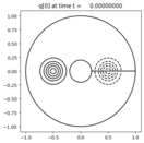
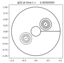
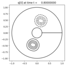
Solve the linear non-conservative advection equation:

\[q_t + u(x,y) q_x + v(x,y) q_y = 0\]

in an annular domain, using a mapped grid.

Here q is the density of some quantity and (u,v) is the velocity field. We take a rotational velocity field: \(u = \cos(\theta), v = \sin(\theta)\).

This is the simplest example that shows how to use a mapped grid in PyClaw. However, it doesn’t use a mapped-grid Riemann solver.

Output:

Source:

#!/usr/bin/env python
# encoding: utf-8
r"""
Advection in an annular domain
==============================

Solve the linear non-conservative advection equation:

.. math::
    q_t + u(x,y) q_x + v(x,y) q_y = 0

in an annular domain, using a mapped grid.

Here q is the density of some quantity and (u,v) is the velocity
field.  We take a rotational velocity field: :math:`u = \cos(\theta), v = \sin(\theta)`.

This is the simplest example that shows how to use a mapped grid in PyClaw.
However, it doesn't use a mapped-grid Riemann solver.
"""
import numpy as np

def mapc2p_annulus(xc, yc):
    """
    Specifies the mapping to curvilinear coordinates.

    Inputs: c_centers = Computational cell centers
                 [array ([Xc1, Xc2, ...]), array([Yc1, Yc2, ...])]

    Output: p_centers = Physical cell centers
                 [array ([Xp1, Xp2, ...]), array([Yp1, Yp2, ...])]
    """  
    p_centers = []

    # Polar coordinates (first coordinate = radius,  second coordinate = theta)
    p_centers.append(xc[:]*np.cos(yc[:]))
    p_centers.append(xc[:]*np.sin(yc[:]))
    
    return p_centers


def qinit(state):
    """
    Initialize with two Gaussian pulses.
    """
    # First gaussian pulse
    A1     = 1.    # Amplitude
    beta1  = 40.   # Decay factor
    r1     = -0.5  # r-coordinate of the center
    theta1 = 0.    # theta-coordinate of the center

    # Second gaussian pulse
    A2     = -1.   # Amplitude
    beta2  = 40.   # Decay factor
    r2     = 0.5   # r-coordinate of the centers
    theta2 = 0.    # theta-coordinate of the centers

    R, Theta = state.grid.p_centers
    state.q[0,:,:] = A1*np.exp(-beta1*(np.square(R-r1) + np.square(Theta-theta1)))\
                   + A2*np.exp(-beta2*(np.square(R-r2) + np.square(Theta-theta2)))


def ghost_velocities_upper(state,dim,t,qbc,auxbc,num_ghost):
    """
    Set the velocities for the ghost cells outside the outer radius of the annulus.
    In the computational domain, these are the cells at the top of the grid.
    """
    grid=state.grid
    if dim == grid.dimensions[0]:
        dx, dy = grid.delta
        R_nodes,Theta_nodes = grid.p_nodes_with_ghost(num_ghost=2)

        auxbc[:,-num_ghost:,:] = edge_velocities_and_area(R_nodes[-num_ghost-1:,:],Theta_nodes[-num_ghost-1:,:],dx,dy)

    else:
        raise Exception('Custom BC for this boundary is not appropriate!')


def ghost_velocities_lower(state,dim,t,qbc,auxbc,num_ghost):
    """
    Set the velocities for the ghost cells outside the inner radius of the annulus.
    In the computational domain, these are the cells at the bottom of the grid.
    """
    grid=state.grid
    if dim == grid.dimensions[0]:
        dx, dy = grid.delta
        R_nodes,Theta_nodes = grid.p_nodes_with_ghost(num_ghost=2)

        auxbc[:,0:num_ghost,:] = edge_velocities_and_area(R_nodes[0:num_ghost+1,:],Theta_nodes[0:num_ghost+1,:],dx,dy)

    else:
        raise Exception('Custom BC for this boundary is not appropriate!')


def edge_velocities_and_area(R_nodes,Theta_nodes,dx,dy):
    """This routine fills in the aux arrays for the problem:

        aux[0,i,j] = u-velocity at left edge of cell (i,j)
        aux[1,i,j] = v-velocity at bottom edge of cell (i,j)
        aux[2,i,j] = physical area of cell (i,j) (relative to area of computational cell)
    """
    mx = R_nodes.shape[0]-1
    my = R_nodes.shape[1]-1
    aux = np.empty((3,mx,my), order='F')

    # Bottom-left corners
    Xp0 = R_nodes[:mx,:my]
    Yp0 = Theta_nodes[:mx,:my]

    # Top-left corners
    Xp1 = R_nodes[:mx,1:]
    Yp1 = Theta_nodes[:mx,1:]

    # Top-right corners
    Xp2 = R_nodes[1:,1:]
    Yp2 = Theta_nodes[1:,1:]

    # Top-left corners
    Xp3 = R_nodes[1:,:my]
    Yp3 = Theta_nodes[1:,:my]

    # Compute velocity component
    aux[0,:mx,:my] = (stream(Xp1,Yp1)- stream(Xp0,Yp0))/dy
    aux[1,:mx,:my] = -(stream(Xp3,Yp3)- stream(Xp0,Yp0))/dx

    # Compute area of the physical element
    area = 1./2.*( (Yp0+Yp1)*(Xp1-Xp0) +
                   (Yp1+Yp2)*(Xp2-Xp1) +
                   (Yp2+Yp3)*(Xp3-Xp2) +
                   (Yp3+Yp0)*(Xp0-Xp3) )
    
    # Compute capa 
    aux[2,:mx,:my] = area/(dx*dy)

    return aux

    
def stream(Xp,Yp):
    """ 
    Calculates the stream function in physical space.
    Clockwise rotation. One full rotation corresponds to 1 (second).
    """
    return np.pi*(Xp**2 + Yp**2)


def setup(use_petsc=False,outdir='./_output',solver_type='classic'):
    from clawpack import riemann

    if use_petsc:
        import clawpack.petclaw as pyclaw
    else:
        from clawpack import pyclaw

    if solver_type == 'classic':
        solver = pyclaw.ClawSolver2D(riemann.vc_advection_2D)
        solver.dimensional_split = False
        solver.transverse_waves = 2
        solver.order = 2
    elif solver_type == 'sharpclaw':
        solver = pyclaw.SharpClawSolver2D(riemann.vc_advection_2D)

    solver.bc_lower[0] = pyclaw.BC.extrap
    solver.bc_upper[0] = pyclaw.BC.extrap
    solver.bc_lower[1] = pyclaw.BC.periodic
    solver.bc_upper[1] = pyclaw.BC.periodic

    solver.aux_bc_lower[0] = pyclaw.BC.custom
    solver.aux_bc_upper[0] = pyclaw.BC.custom
    solver.user_aux_bc_lower = ghost_velocities_lower
    solver.user_aux_bc_upper = ghost_velocities_upper
    solver.aux_bc_lower[1] = pyclaw.BC.periodic
    solver.aux_bc_upper[1] = pyclaw.BC.periodic

    solver.dt_initial = 0.1
    solver.cfl_max = 0.5
    solver.cfl_desired = 0.4

    solver.limiters = pyclaw.limiters.tvd.vanleer

    r_lower = 0.2
    r_upper = 1.0
    m_r = 40

    theta_lower = 0.0
    theta_upper = np.pi*2.0
    m_theta = 120

    r     = pyclaw.Dimension(r_lower,r_upper,m_r,name='r')
    theta = pyclaw.Dimension(theta_lower,theta_upper,m_theta,name='theta')
    domain = pyclaw.Domain([r,theta])
    domain.grid.mapc2p = mapc2p_annulus
    domain.grid.num_ghost = solver.num_ghost

    num_eqn = 1
    state = pyclaw.State(domain,num_eqn)

    qinit(state)

    dx, dy = state.grid.delta
    p_corners = state.grid.p_nodes
    state.aux = edge_velocities_and_area(p_corners[0],p_corners[1],dx,dy)
    state.index_capa = 2 # aux[2,:,:] holds the capacity function

    claw = pyclaw.Controller()
    claw.tfinal = 1.0
    claw.solution = pyclaw.Solution(state,domain)
    claw.solver = solver
    claw.outdir = outdir
    claw.setplot = setplot
    claw.keep_copy = True

    return claw


def setplot(plotdata):
    """ 
    Plot solution using VisClaw.
    """
    from clawpack.pyclaw.examples.advection_2d_annulus.mapc2p import mapc2p
    import numpy as np
    from clawpack.visclaw import colormaps

    plotdata.clearfigures()  # clear any old figures,axes,items data
    plotdata.mapc2p = mapc2p
    
    # Figure for contour plot
    plotfigure = plotdata.new_plotfigure(name='contour', figno=0)

    # Set up for axes in this figure:
    plotaxes = plotfigure.new_plotaxes()
    plotaxes.xlimits = 'auto'
    plotaxes.ylimits = 'auto'
    plotaxes.title = 'q[0]'
    plotaxes.scaled = True

    # Set up for item on these axes:
    plotitem = plotaxes.new_plotitem(plot_type='2d_contour')
    plotitem.plot_var = 0
    plotitem.contour_levels = np.linspace(-0.9, 0.9, 10)
    plotitem.contour_colors = 'k'
    plotitem.patchedges_show = 1
    plotitem.MappedGrid = True

    # Figure for pcolor plot
    plotfigure = plotdata.new_plotfigure(name='q[0]', figno=1)

    # Set up for axes in this figure:
    plotaxes = plotfigure.new_plotaxes()
    plotaxes.xlimits = 'auto'
    plotaxes.ylimits = 'auto'
    plotaxes.title = 'q[0]'
    plotaxes.scaled = True

    # Set up for item on these axes:
    plotitem = plotaxes.new_plotitem(plot_type='2d_pcolor')
    plotitem.plot_var = 0
    plotitem.pcolor_cmap = colormaps.red_yellow_blue
    plotitem.pcolor_cmin = -1.
    plotitem.pcolor_cmax = 1.
    plotitem.add_colorbar = True
    plotitem.MappedGrid = True


    return plotdata

 
if __name__=="__main__":
    from clawpack.pyclaw.util import run_app_from_main
    output = run_app_from_main(setup,setplot)