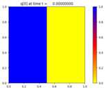
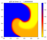
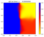
2-dimensional advection-reaction
Output:
Source:
#!/usr/bin/env python
# encoding: utf-8
r"""
Advection-reaction in 2D
========================
Solve the 2D advection-reaction problem

.. math::
    p_t + u(x,y,t) p_x + v(x,y,t) p_y = \epsilon q \\
    q_t + u(x,y,t) q_x + v(x,y,t) q_y = \epsilon p

Note that the left hand side of this system is the non-conservative transport
equation for p and q.  The Riemann solver assumes that velocities are specified
at cell edges.

This example also shows how to use your own Riemann solver.
"""

import numpy as np
import os

try:
    from clawpack.pyclaw.examples.advection_reaction_2d import advection_2d
except ImportError:
    this_dir = os.path.dirname(__file__)
    if this_dir == '':
        this_dir = os.path.abspath('.')
    import subprocess
    cmd = "make -C "+this_dir
    proc = subprocess.Popen("make -C "+this_dir+"/", shell=True, stdout = subprocess.PIPE)
    proc.wait()
    try:
        # Now try to import again
        from clawpack.pyclaw.examples.advection_reaction_2d import advection_2d
    except ImportError:
        raise


t_period = 4.0
epsilon = 0.1

def source_step(solver,state,dt):
    "Integrate the source term over one step."
    qq = state.q.copy()
    state.q[0,:,:] = state.q[0,:,:] + epsilon*dt*qq[1,:,:]
    state.q[1,:,:] = state.q[1,:,:] + epsilon*dt*qq[0,:,:]


def psi(x,y):
    "Velocity field potential."
    return (np.sin(np.pi*x))**2 * (np.sin(np.pi*y))**2 / np.pi

def set_velocities(solver,state):
    "Update velocity field for current time."
    v_t = np.cos(2 * np.pi * (state.t + solver.dt/2) / t_period)
    X, Y = state.grid.p_nodes
    dx, dy = state.grid.delta
    # u(x_(i-1/2),y_j)
    state.aux[0,:,:] = - ( psi(X[:-1,1:],Y[:-1,1:]) - psi(X[:-1,:-1],Y[:-1,:-1]) ) / dy
    # v(x_i,y_(j-1/2))
    state.aux[1,:,:] =   ( psi(X[1:,:-1],Y[1:,:-1]) - psi(X[:-1,:-1],Y[:-1,:-1]) ) / dx
    state.aux[:] = v_t * state.aux[:]


def setup(outdir='./_output'):
    from clawpack import pyclaw
    from clawpack.pyclaw.examples.advection_reaction_2d import advection_2d

    solver = pyclaw.ClawSolver2D(advection_2d)
    # Use dimensional splitting since no transverse solver is defined
    solver.dimensional_split = 1

    solver.all_bcs = pyclaw.BC.extrap
    solver.aux_bc_lower[0] = pyclaw.BC.extrap
    solver.aux_bc_upper[0] = pyclaw.BC.extrap
    solver.aux_bc_lower[1] = pyclaw.BC.extrap
    solver.aux_bc_upper[1] = pyclaw.BC.extrap

    domain = pyclaw.Domain( (0.,0.), (1.,1.), (100,100) )
    solver.num_eqn = 2
    solver.num_waves = 1
    num_aux = 2
    state = pyclaw.State(domain, solver.num_eqn, num_aux)

    Xe, Ye = domain.grid.p_nodes
    Xc, Yc = domain.grid.p_centers
    dx, dy = domain.grid.delta

    # Edge velocities
    # u(x_(i-1/2),y_j)
    state.aux[0,:,:] = - ( psi(Xe[:-1,1:],Ye[:-1,1:]) - psi(Xe[:-1,:-1],Ye[:-1,:-1]) ) / dy
    # v(x_i,y_(j-1/2))
    state.aux[1,:,:] =   ( psi(Xe[1:,:-1],Ye[1:,:-1]) - psi(Xe[:-1,:-1],Ye[:-1,:-1]) ) / dx

    solver.before_step = set_velocities
    solver.step_source = source_step
    solver.source_split = 1

    state.q[0,:,:] = (Xc <= 0.5)
    state.q[1,:,:] = (Yc <= 0.5)

    claw = pyclaw.Controller()
    claw.tfinal = t_period
    claw.solution = pyclaw.Solution(state, domain)
    claw.solver = solver
    claw.keep_copy = True
    claw.outdir = outdir
    if outdir == '':
        claw.output_format = None
    claw.setplot = setplot

    return claw

def setplot(plotdata):
    """
    Plot solution using VisClaw.
    """
    from clawpack.visclaw import colormaps

    plotdata.clearfigures()  # clear any old figures,axes,items data

    # Figure for pcolor plot
    plotfigure = plotdata.new_plotfigure(name='q[0]', figno=0)

    # Set up for axes in this figure:
    plotaxes = plotfigure.new_plotaxes()
    plotaxes.title = 'q[0]'
    plotaxes.scaled = True

    # Set up for item on these axes:
    plotitem = plotaxes.new_plotitem(plot_type='2d_pcolor')
    plotitem.plot_var = 0
    plotitem.pcolor_cmap = colormaps.yellow_red_blue
    plotitem.pcolor_cmin = 0.0
    plotitem.pcolor_cmax = 1.0
    plotitem.add_colorbar = True

    # Figure for contour plot
    plotfigure = plotdata.new_plotfigure(name='q[1]', figno=1)

    # Set up for axes in this figure:
    plotaxes = plotfigure.new_plotaxes()
    plotaxes.title = 'q[1]'

    # Set up for item on these axes:
    plotitem = plotaxes.new_plotitem(plot_type='2d_pcolor')
    plotitem.plot_var = 1
    plotitem.pcolor_cmin = 0.0
    plotitem.pcolor_cmax = 1.0
    plotitem.add_colorbar = True

    return plotdata

if __name__=="__main__":
    from clawpack.pyclaw.util import run_app_from_main
    output = run_app_from_main(setup,setplot)