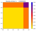
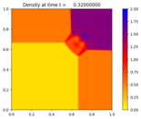
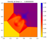
2-dimensional Euler equations
Output:
Source:
#!/usr/bin/env python
# encoding: utf-8
r"""
Euler 2D Quadrants example
==========================

Simple example solving the Euler equations of compressible fluid dynamics:

.. math::
    \rho_t + (\rho u)_x + (\rho v)_y & = 0 \\
    (\rho u)_t + (\rho u^2 + p)_x + (\rho uv)_y & = 0 \\
    (\rho v)_t + (\rho uv)_x + (\rho v^2 + p)_y & = 0 \\
    E_t + (u (E + p) )_x + (v (E + p))_y & = 0.

Here :math:`\rho` is the density, (u,v) is the velocity, and E is the total energy.
The initial condition is one of the 2D Riemann problems from the paper of
Liska and Wendroff.

"""
from clawpack import riemann
from clawpack.riemann.euler_4wave_2D_constants import density, x_momentum, y_momentum, \
        energy, num_eqn
from clawpack.visclaw import colormaps

def setplot(plotdata):
    r"""Plotting settings

    Should plot two figures both of density.

    """


    plotdata.clearfigures()  # clear any old figures,axes,items data

    # Figure for density - pcolor
    plotfigure = plotdata.new_plotfigure(name='Density', figno=0)

    # Set up for axes in this figure:
    plotaxes = plotfigure.new_plotaxes()
    plotaxes.xlimits = 'auto'
    plotaxes.ylimits = 'auto'
    plotaxes.scaled = True
    plotaxes.title = 'Density'

    # Set up for item on these axes:
    plotitem = plotaxes.new_plotitem(plot_type='2d_pcolor')
    plotitem.plot_var = density
    plotitem.pcolor_cmap = colormaps.yellow_red_blue
    plotitem.pcolor_cmin = 0.
    plotitem.pcolor_cmax = 2.
    plotitem.add_colorbar = True

    # Figure for density - Schlieren
    plotfigure = plotdata.new_plotfigure(name='Schlieren', figno=1)

    # Set up for axes in this figure:
    plotaxes = plotfigure.new_plotaxes()
    plotaxes.xlimits = 'auto'
    plotaxes.ylimits = 'auto'
    plotaxes.title = 'Density'
    plotaxes.scaled = True      # so aspect ratio is 1

    # Set up for item on these axes:
    plotitem = plotaxes.new_plotitem(plot_type='2d_schlieren')
    plotitem.schlieren_cmin = 0.0
    plotitem.schlieren_cmax = 1.0
    plotitem.plot_var = density
    plotitem.add_colorbar = False

    return plotdata


def setup(use_petsc=False,riemann_solver='roe'):
    if use_petsc:
        import clawpack.petclaw as pyclaw
    else:
        from clawpack import pyclaw

    if riemann_solver.lower() == 'roe':
        solver = pyclaw.ClawSolver2D(riemann.euler_4wave_2D)
        solver.transverse_waves = 2
    elif riemann_solver.lower() == 'hlle':
        solver = pyclaw.ClawSolver2D(riemann.euler_hlle_2D)
        solver.transverse_waves = 0
        solver.cfl_desired = 0.4
        solver.cfl_max = 0.5
    solver.all_bcs = pyclaw.BC.extrap

    domain = pyclaw.Domain([0.,0.],[1.,1.],[100,100])
    solution = pyclaw.Solution(num_eqn,domain)
    gamma = 1.4
    solution.problem_data['gamma']  = gamma

    # Set initial data
    xx, yy = domain.grid.p_centers
    l = xx < 0.8
    r = xx >= 0.8
    b = yy < 0.8
    t = yy >= 0.8
    solution.q[density,...] = 1.5 * r * t + 0.532258064516129 * l * t          \
                                          + 0.137992831541219 * l * b          \
                                          + 0.532258064516129 * r * b
    u = 0.0 * r * t + 1.206045378311055 * l * t                                \
                    + 1.206045378311055 * l * b                                \
                    + 0.0 * r * b
    v = 0.0 * r * t + 0.0 * l * t                                              \
                    + 1.206045378311055 * l * b                                \
                    + 1.206045378311055 * r * b
    p = 1.5 * r * t + 0.3 * l * t + 0.029032258064516 * l * b + 0.3 * r * b
    solution.q[x_momentum,...] = solution.q[density, ...] * u
    solution.q[y_momentum,...] = solution.q[density, ...] * v
    solution.q[energy,...] = 0.5 * solution.q[density,...]*(u**2 + v**2) + p / (gamma - 1.0)

    claw = pyclaw.Controller()
    claw.tfinal = 0.8
    claw.num_output_times = 10
    claw.solution = solution
    claw.solver = solver

    claw.output_format = 'ascii'
    claw.outdir = "./_output"
    claw.keep_copy = True
    claw.setplot = setplot

    return claw

if __name__ == "__main__":
    from clawpack.pyclaw.util import run_app_from_main
    output = run_app_from_main(setup, setplot)