2-dimensional Euler equations
Output:
Source:
#!/usr/bin/env python
# encoding: utf-8
r"""
Compressible Euler flow in cylindrical symmetry
===============================================
Solve the Euler equations of compressible fluid dynamics in 2D r-z coordinates:
.. math::
\rho_t + (\rho u)_x + (\rho v)_y & = - \rho v / r \\
(\rho u)_t + (\rho u^2 + p)_x + (\rho uv)_y & = -\rho u v / r \\
(\rho v)_t + (\rho uv)_x + (\rho v^2 + p)_y & = - \rho v^2 / r \\
E_t + (u (E + p) )_x + (v (E + p))_y & = - (E + p) v / r.
Here :math:`\rho` is the density, (u,v) is the velocity, and E is the total energy.
The radial coordinate is denoted by r.
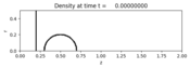
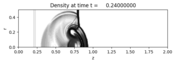
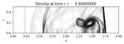
The problem involves a planar shock wave impacting a spherical low-density bubble.
The problem is 3-dimensional but has been reduced to two dimensions using
cylindrical symmetry.
This problem demonstrates:
- how to incorporate source (non-hyperbolic) terms using both Classic and SharpClaw solvers
- how to impose a custom boundary condition
- how to use the auxiliary array for spatially-varying coefficients
"""
import numpy as np
from clawpack import riemann
from clawpack.riemann.euler_5wave_2D_constants import density, x_momentum, y_momentum, \
energy, num_eqn
gamma = 1.4 # Ratio of specific heats
x0=0.5; y0=0.; r0=0.2
def ycirc(x,ymin,ymax):
if ((x-x0)**2)<(r0**2):
return max(min(y0 + np.sqrt(r0**2-(x-x0)**2),ymax) - ymin,0.)
else:
return 0
def qinit(state,rhoin=0.1,pinf=5.):
from scipy import integrate
gamma1 = gamma - 1.
grid = state.grid
rhoout = 1.
pout = 1.
pin = 1.
xshock = 0.2
rinf = (gamma1 + pinf*(gamma+1.))/ ((gamma+1.) + gamma1*pinf)
vinf = 1./np.sqrt(gamma) * (pinf - 1.) / np.sqrt(0.5*((gamma+1.)/gamma) * pinf+0.5*gamma1/gamma)
einf = 0.5*rinf*vinf**2 + pinf/gamma1
X, Y = grid.p_centers
r = np.sqrt((X-x0)**2 + (Y-y0)**2)
#First set the values for the cells that don't intersect the bubble boundary
state.q[0,:,:] = rinf*(X<xshock) + rhoin*(r<=r0) + rhoout*(r>r0)*(X>=xshock)
state.q[1,:,:] = rinf*vinf*(X<xshock)
state.q[2,:,:] = 0.
state.q[3,:,:] = einf*(X<xshock) + (pin*(r<=r0) + pout*(r>r0)*(X>=xshock))/gamma1
state.q[4,:,:] = 1.*(r<=r0)
#Now compute average density for the cells on the edge of the bubble
d2 = np.linalg.norm(state.grid.delta)/2.
dx = state.grid.delta[0]
dy = state.grid.delta[1]
dx2 = state.grid.delta[0]/2.
dy2 = state.grid.delta[1]/2.
for i in range(state.q.shape[1]):
for j in range(state.q.shape[2]):
ydown = Y[i,j]-dy2
yup = Y[i,j]+dy2
if abs(r[i,j]-r0)<d2:
infrac,abserr = integrate.quad(ycirc,X[i,j]-dx2,X[i,j]+dx2,args=(ydown,yup),epsabs=1.e-8,epsrel=1.e-5)
infrac=infrac/(dx*dy)
state.q[0,i,j] = rhoin*infrac + rhoout*(1.-infrac)
state.q[3,i,j] = (pin*infrac + pout*(1.-infrac))/gamma1
state.q[4,i,j] = 1.*infrac
def auxinit(state):
"""
aux[1,i,j] = radial coordinate of cell centers for cylindrical source terms
"""
y = state.grid.y.centers
for j,r in enumerate(y):
state.aux[0,:,j] = r
def incoming_shock(state,dim,t,qbc,auxbc,num_ghost):
"""
Incoming shock at left boundary.
"""
gamma1 = gamma - 1.
pinf=5.
rinf = (gamma1 + pinf*(gamma+1.))/ ((gamma+1.) + gamma1*pinf)
vinf = 1./np.sqrt(gamma) * (pinf - 1.) / np.sqrt(0.5*((gamma+1.)/gamma) * pinf+0.5*gamma1/gamma)
einf = 0.5*rinf*vinf**2 + pinf/gamma1
for i in range(num_ghost):
qbc[0,i,...] = rinf
qbc[1,i,...] = rinf*vinf
qbc[2,i,...] = 0.
qbc[3,i,...] = einf
qbc[4,i,...] = 0.
def step_Euler_radial(solver,state,dt):
"""
Geometric source terms for Euler equations with cylindrical symmetry.
Integrated using a 2-stage, 2nd-order Runge-Kutta method.
This is a Clawpack-style source term routine, which approximates
the integral of the source terms over a step.
"""
dt2 = dt/2.
q = state.q
rad = state.aux[0,:,:]
rho = q[0,:,:]
u = q[1,:,:]/rho
v = q[2,:,:]/rho
press = (gamma - 1.) * (q[3,:,:] - 0.5*rho*(u**2 + v**2))
qstar = np.empty(q.shape)
qstar[0,:,:] = q[0,:,:] - dt2/rad * q[2,:,:]
qstar[1,:,:] = q[1,:,:] - dt2/rad * rho*u*v
qstar[2,:,:] = q[2,:,:] - dt2/rad * rho*v*v
qstar[3,:,:] = q[3,:,:] - dt2/rad * v * (q[3,:,:] + press)
rho = qstar[0,:,:]
u = qstar[1,:,:]/rho
v = qstar[2,:,:]/rho
press = (gamma - 1.) * (qstar[3,:,:] - 0.5*rho*(u**2 + v**2))
q[0,:,:] = q[0,:,:] - dt/rad * qstar[2,:,:]
q[1,:,:] = q[1,:,:] - dt/rad * rho*u*v
q[2,:,:] = q[2,:,:] - dt/rad * rho*v*v
q[3,:,:] = q[3,:,:] - dt/rad * v * (qstar[3,:,:] + press)
def dq_Euler_radial(solver,state,dt):
"""
Geometric source terms for Euler equations with radial symmetry.
This is a SharpClaw-style source term routine, which returns
the value of the source terms.
"""
q = state.q
rad = state.aux[0,:,:]
rho = q[0,:,:]
u = q[1,:,:]/rho
v = q[2,:,:]/rho
press = (gamma - 1.) * (q[3,:,:] - 0.5*rho*(u**2 + v**2))
dq = np.empty(q.shape)
dq[0,:,:] = -dt/rad * q[2,:,:]
dq[1,:,:] = -dt/rad * rho*u*v
dq[2,:,:] = -dt/rad * rho*v*v
dq[3,:,:] = -dt/rad * v * (q[3,:,:] + press)
dq[4,:,:] = 0
return dq
def setup(use_petsc=False,solver_type='classic', outdir='_output', kernel_language='Fortran',
disable_output=False, mx=320, my=80, tfinal=0.6, num_output_times = 10):
if use_petsc:
import clawpack.petclaw as pyclaw
else:
from clawpack import pyclaw
if solver_type=='sharpclaw':
solver = pyclaw.SharpClawSolver2D(riemann.euler_5wave_2D)
solver.dq_src = dq_Euler_radial
solver.weno_order = 5
solver.lim_type = 2
else:
solver = pyclaw.ClawSolver2D(riemann.euler_5wave_2D)
solver.step_source = step_Euler_radial
solver.source_split = 1
solver.limiters = [4,4,4,4,2]
solver.cfl_max = 0.5
solver.cfl_desired = 0.45
x = pyclaw.Dimension(0.0,2.0,mx,name='x')
y = pyclaw.Dimension(0.0,0.5,my,name='y')
domain = pyclaw.Domain([x,y])
num_aux=1
state = pyclaw.State(domain,num_eqn,num_aux)
state.problem_data['gamma']= gamma
qinit(state)
auxinit(state)
solver.user_bc_lower = incoming_shock
solver.bc_lower[0]=pyclaw.BC.custom
solver.bc_upper[0]=pyclaw.BC.extrap
solver.bc_lower[1]=pyclaw.BC.wall
solver.bc_upper[1]=pyclaw.BC.extrap
#Aux variable in ghost cells doesn't matter
solver.aux_bc_lower[0]=pyclaw.BC.extrap
solver.aux_bc_upper[0]=pyclaw.BC.extrap
solver.aux_bc_lower[1]=pyclaw.BC.extrap
solver.aux_bc_upper[1]=pyclaw.BC.extrap
claw = pyclaw.Controller()
claw.solution = pyclaw.Solution(state,domain)
claw.solver = solver
claw.keep_copy = True
if disable_output or outdir is None:
claw.output_format = None
claw.tfinal = tfinal
claw.num_output_times = num_output_times
claw.outdir = outdir
claw.setplot = setplot
return claw
def setplot(plotdata):
"""
Plot solution using VisClaw.
"""
from clawpack.visclaw import colormaps
plotdata.clearfigures() # clear any old figures,axes,items data
# Pressure plot
plotfigure = plotdata.new_plotfigure(name='Density', figno=0)
plotaxes = plotfigure.new_plotaxes()
plotaxes.title = 'Density'
plotaxes.scaled = True # so aspect ratio is 1
plotaxes.afteraxes = label_axes
plotitem = plotaxes.new_plotitem(plot_type='2d_schlieren')
plotitem.plot_var = 0
plotitem.add_colorbar = False
# Tracer plot
plotfigure = plotdata.new_plotfigure(name='Tracer', figno=1)
plotaxes = plotfigure.new_plotaxes()
plotaxes.title = 'Tracer'
plotaxes.scaled = True # so aspect ratio is 1
plotaxes.afteraxes = label_axes
plotitem = plotaxes.new_plotitem(plot_type='2d_pcolor')
plotitem.pcolor_cmin = 0.
plotitem.pcolor_cmax=1.0
plotitem.plot_var = 4
plotitem.pcolor_cmap = colormaps.yellow_red_blue
plotitem.add_colorbar = False
# Energy plot
plotfigure = plotdata.new_plotfigure(name='Energy', figno=2)
plotaxes = plotfigure.new_plotaxes()
plotaxes.title = 'Energy'
plotaxes.scaled = True # so aspect ratio is 1
plotaxes.afteraxes = label_axes
plotitem = plotaxes.new_plotitem(plot_type='2d_pcolor')
plotitem.pcolor_cmin = 2.
plotitem.pcolor_cmax=18.0
plotitem.plot_var = 3
plotitem.pcolor_cmap = colormaps.yellow_red_blue
plotitem.add_colorbar = False
return plotdata
def label_axes(current_data):
import matplotlib.pyplot as plt
plt.xlabel('z')
plt.ylabel('r')
if __name__=="__main__":
from clawpack.pyclaw.util import run_app_from_main
output = run_app_from_main(setup,setplot)