1-dimensional nonlinear elasticity

Output:

Source:

#!/usr/bin/env python
# encoding: utf-8
r"""
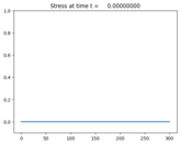
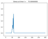
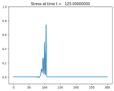
Solitary wave formation in periodic nonlinear elastic media
===========================================================

Solve a one-dimensional nonlinear elasticity system:

.. math::
    \epsilon_t + u_x & = 0 \\
    (\rho(x) u)_t + \sigma(\epsilon,x)_x & = 0.

Here :math:`\epsilon` is the strain, :math:`\sigma` is the stress, 
u is the velocity, and :math:`\rho(x)` is the density.  
We take the stress-strain relation :math:`\sigma = e^{K(x)\epsilon}-1`;
:math:`K(x)` is the linearized bulk modulus.
Note that the density and bulk modulus may depend explicitly on x.

The problem solved here is based on [LeVYon03]_.  An initial hump
evolves into two trains of solitary waves.

"""
import numpy as np

def qinit(state,ic=2,a2=1.0,xupper=600.):
    x = state.grid.x.centers
    
    if ic==1: #Zero ic
        state.q[:,:] = 0.
    elif ic==2:
        # Gaussian
        sigma = a2*np.exp(-((x-xupper/2.)/10.)**2.)
        state.q[0,:] = np.log(sigma+1.)/state.aux[1,:]
        state.q[1,:] = 0.


def setaux(x,rhoB=4,KB=4,rhoA=1,KA=1,alpha=0.5,xlower=0.,xupper=600.,bc=2):
    aux = np.empty([3,len(x)],order='F')
    xfrac = x-np.floor(x)
    #Density:
    aux[0,:] = rhoA*(xfrac<alpha)+rhoB*(xfrac>=alpha)
    #Bulk modulus:
    aux[1,:] = KA  *(xfrac<alpha)+KB  *(xfrac>=alpha)
    aux[2,:] = 0. # not used
    return aux

    
def b4step(solver,state):
    #Reverse velocity at trtime
    #Note that trtime should be an output point
    if state.t>=state.problem_data['trtime']-1.e-10 and not state.problem_data['trdone']:
        #print 'Time reversing'
        state.q[1,:]=-state.q[1,:]
        state.q=state.q
        state.problem_data['trdone']=True
        if state.t>state.problem_data['trtime']:
            print('WARNING: trtime is '+str(state.problem_data['trtime'])+\
                ' but velocities reversed at time '+str(state.t))
    #Change to periodic BCs after initial pulse 
    if state.t>5*state.problem_data['tw1'] and solver.bc_lower[0]==0:
        solver.bc_lower[0]=2
        solver.bc_upper[0]=2
        solver.aux_bc_lower[0]=2
        solver.aux_bc_upper[0]=2


def zero_bc(state,dim,t,qbc,auxbc,num_ghost):
    """Set everything to zero"""
    if dim.on_upper_boundary:
        qbc[:,-num_ghost:]=0.

def moving_wall_bc(state,dim,t,qbc,auxbc,num_ghost):
    """Initial pulse generated at left boundary by prescribed motion"""
    if dim.on_lower_boundary:
        qbc[0,:num_ghost]=qbc[0,num_ghost] 
        t=state.t; t1=state.problem_data['t1']; tw1=state.problem_data['tw1']
        a1=state.problem_data['a1'];
        t0 = (t-t1)/tw1
        if abs(t0)<=1.: vwall = -a1*(1.+np.cos(t0*np.pi))
        else: vwall=0.
        for ibc in range(num_ghost-1):
            qbc[1,num_ghost-ibc-1] = 2*vwall*state.aux[1,ibc] - qbc[1,num_ghost+ibc]



def setup(use_petsc=0,kernel_language='Fortran',solver_type='classic',outdir='./_output'):
    from clawpack import riemann

    if use_petsc:
        import clawpack.petclaw as pyclaw
    else:
        from clawpack import pyclaw

    if kernel_language=='Python':
        rs = riemann.nonlinear_elasticity_1D_py.nonlinear_elasticity_1D
    elif kernel_language=='Fortran':
        rs = riemann.nonlinear_elasticity_fwave_1D

    if solver_type=='sharpclaw':
        solver = pyclaw.SharpClawSolver1D(rs)
        solver.char_decomp=0
    else:
        solver = pyclaw.ClawSolver1D(rs)

    solver.kernel_language = kernel_language

    solver.bc_lower[0] = pyclaw.BC.custom
    solver.bc_upper[0] = pyclaw.BC.extrap

    #Use the same BCs for the aux array
    solver.aux_bc_lower[0] = pyclaw.BC.extrap
    solver.aux_bc_upper[0] = pyclaw.BC.extrap

    xlower=0.0; xupper=300.0
    cells_per_layer=12; mx=int(round(xupper-xlower))*cells_per_layer
    x = pyclaw.Dimension(xlower,xupper,mx,name='x')
    domain = pyclaw.Domain(x)
    state = pyclaw.State(domain,solver.num_eqn,num_aux=3)
    state.problem_data['stress_relation'] = 'exponential'

    #Set global parameters
    alpha = 0.5
    KA    = 1.0
    KB    = 4.0
    rhoA  = 1.0
    rhoB  = 4.0
    state.problem_data = {}
    state.problem_data['t1']    = 10.0
    state.problem_data['tw1']   = 10.0
    state.problem_data['a1']    = 0.1
    state.problem_data['alpha'] = alpha
    state.problem_data['KA'] = KA
    state.problem_data['KB'] = KB
    state.problem_data['rhoA'] = rhoA
    state.problem_data['rhoB'] = rhoB
    state.problem_data['trtime'] = 999999999.0
    state.problem_data['trdone'] = False

    #Initialize q and aux
    xc=state.grid.x.centers
    state.aux[:,:] = setaux(xc,rhoB,KB,rhoA,KA,alpha,xlower=xlower,xupper=xupper)
    qinit(state,ic=1,a2=1.0,xupper=xupper)

    tfinal=500.; num_output_times = 20;

    solver.max_steps = 5000000
    solver.fwave = True 
    solver.before_step = b4step 
    solver.user_bc_lower=moving_wall_bc
    solver.user_bc_upper=zero_bc

    claw = pyclaw.Controller()
    claw.output_style = 1
    claw.num_output_times = num_output_times
    claw.tfinal = tfinal
    claw.solution = pyclaw.Solution(state,domain)
    claw.solver = solver
    claw.setplot = setplot
    claw.keep_copy = True

    return claw


#--------------------------
def setplot(plotdata):
#--------------------------
    """ 
    Specify what is to be plotted at each frame.
    Input:  plotdata, an instance of visclaw.data.ClawPlotData.
    Output: a modified version of plotdata.
    """ 
    plotdata.clearfigures()  # clear any old figures,axes,items data

    # Figure for q[0]
    plotfigure = plotdata.new_plotfigure(name='Stress', figno=1)

    # Set up for axes in this figure:
    plotaxes = plotfigure.new_plotaxes()
    plotaxes.title = 'Stress'
    plotaxes.ylimits = [-0.1,1.0]

    # Set up for item on these axes:
    plotitem = plotaxes.new_plotitem(plot_type='1d_plot')
    plotitem.plot_var = stress
    plotitem.kwargs = {'linewidth':2}
    
    # Figure for q[1]
    plotfigure = plotdata.new_plotfigure(name='Velocity', figno=2)

    # Set up for axes in this figure:
    plotaxes = plotfigure.new_plotaxes()
    plotaxes.xlimits = 'auto'
    plotaxes.ylimits = [-.5,0.1]
    plotaxes.title = 'Velocity'

    # Set up for item on these axes:
    plotitem = plotaxes.new_plotitem(plot_type='1d_plot')
    plotitem.plot_var = velocity
    plotitem.kwargs = {'linewidth':2}
    
    return plotdata

 
def velocity(current_data):
    """Compute velocity from strain and momentum"""
    aux=setaux(current_data.x,rhoB=4,KB=4)
    velocity = current_data.q[1,:]/aux[0,:]
    return velocity

def stress(current_data):
    """Compute stress from strain and momentum"""
    from clawpack.riemann.nonlinear_elasticity_1D_py import sigma 
    aux=setaux(current_data.x)
    epsilon = current_data.q[0,:]
    stress = sigma(current_data.q,aux,{'stress_relation':'exponential'})
    return stress

if __name__=="__main__":
    from clawpack.pyclaw.util import run_app_from_main
    output = run_app_from_main(setup,setplot)