Understanding Pyclaw Classes
Contents
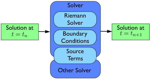
Flow of a Pyclaw Simulation
The basic idea of a pyclaw simulation is to construct a
Solution object, hand it to a
Solver object, and request a solution at a new
time. The solver will take whatever steps are necessary to evolve the solution
to the requested time.
The bulk of the work in order to run a simulation then is the creation and
setup of the appropriate Domain, State,
Solution, and Solver
objects needed to evolve the solution to the requested time.
Creation of a Pyclaw Solution
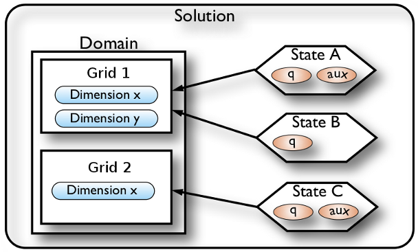
A Pyclaw Solution is a container for a collection of
Domain and State designed with a
view to future support of adaptive mesh refinement and multi-block simulations. The Solution
object keeps track of a list of State objects
and controls the overall input and output of the entire collection of
State objects. Each
State object inhabits a Grid, composed of
Dimension objects that define the extents
of the Domain. Multiple states can inhabit the same
grid, but each State inhabits a single grid.
The process needed to create a Solution object then
follows from the bottom up.
>>> from clawpack import pyclaw
>>> x = pyclaw.Dimension('x', -1.0, 1.0, 200)
>>> y = pyclaw.Dimension('y', 0.0, 1.0, 100)
This code creates two dimensions, a dimension x on the interval
[-1.0, 1.0] with \(200\) grid points and a dimension y on the interval
[0.0, 1.0] with \(100\) grid points.
Note
Many of the attributes of a Dimension
object are set automatically so make sure that the values you want are set
by default. Please refer to the Dimension
classes definition for what the default values are.
Next we have to create a Domain object that will
contain our dimensions objects.
>>> domain = pyclaw.Domain([x,y])
>>> num_eqn = 2
>>> state = pyclaw.State(domain,num_eqn)
Here we create a domain with the dimensions we created earlier to make a single 2D
Domain object. Then we set the number of equations the State
will represent to 2. Finally, we create a State that inhabits
this domain. As before, many of the attributes of the Domain
and State objects are set automatically.
We now need to set the initial condition q and possibly aux to the correct
values.
>>> import numpy as np
>>> sigma = 0.2
>>> omega = np.pi
>>> Y,X = np.meshgrid(state.grid.y.centers,state.grid.x.centers)
>>> r = np.sqrt(X**2 + Y**2)
>>> state.q[0,:] = np.cos(omega * r)
>>> state.q[1,:] = np.exp(-r**2 / sigma**2)
We now have initialized the first entry of q to a cosine function
evaluated at the cell centers and the second entry of q to a gaussian, again
evaluated at the grid cell centers.
Many Riemann solvers also require information about the problem we are going
to run which happen to be grid properties such as the impedence \(Z\) and
speed of sound \(c\) for linear acoustics. We can set these values in the
problem_data dictionary in one of two ways. The first way is to set them
directly as in:
>>> state.problem_data['c'] = 1.0
>>> state.problem_data['Z'] = 0.25
If you’re using a Fortran Riemann solver, these values will automatically get copied to the corresponding variables in the cparam common block of the Riemann solver. This is done in solver.setup(), which calls state.set_cparam().
Last we have to put our State object into a
Solution object to complete the process. In this
case, since we are not using adaptive mesh refinement or a multi-block
algorithm, we do not have multiple grids.
>>> sol = pyclaw.Solution(state,domain)
We now have a solution ready to be evolved in a
Solver object.
Creation of a Pyclaw Solver
A Pyclaw Solver can represent many different
types of solvers; here we will use a 1D, classic Clawpack type of
solver. This solver is defined in the solver module.
First we import the particular solver we want and create it with the default configuration.
>>> solver = pyclaw.ClawSolver1D()
>>> solver.bc_lower[0] = pyclaw.BC.periodic
>>> solver.bc_upper[0] = pyclaw.BC.periodic
Next we need to tell the solver which Riemann solver to use from the
Riemann Solver Package. We can always
check what Riemann solvers are available to use via the riemann
module. Once we have picked one out, we pass it to the solver via:
>>> from clawpack import riemann
>>> solver.rp = riemann.acoustics_1D
In this case we have decided to use the 1D linear acoustics Riemann solver. You
can also set your own solver by importing the module that contains it and
setting it directly to the rp attribute of the particular object in the class
ClawSolver1D.
>>> import my_rp_module
>>> solver.rp = my_rp_module.my_acoustics_rp
Last we finish up by specifying solver options, if we want to override the defaults. For instance, we might want to specify a particular limiter
>>> solver.limiters = pyclaw.limiters.tvd.vanleer
If we wanted to control the simulation we could at this point by issuing the following commands:
>>> solver.evolve_to_time(sol,1.0)
This would evolve our solution sol to t = 1.0 but we are then
responsible for all output and other setup considerations.
Creating and Running a Simulation with Controller
The Controller coordinates the output and setup of
a run with the same parameters as the classic Clawpack. In order to have it
control a run, we need only to create the controller, assign it a solver and
initial condition, and call the run()
method.
>>> from pyclaw.controller import Controller

>>> claw = Controller()
>>> claw.solver = solver
>>> claw.solutions = sol
Here we have imported and created the Controller
class, assigned the Solver and
Solution.
These next commands setup the type of output the controller will output. The parameters are similar to the ones found in the classic clawpack claw.data format.
>>> claw.output_style = 1
>>> claw.num_output_times = 10
>>> claw.tfinal = 1.0
When we are ready to run the simulation, we can call the
run() method. It will then run the
simulation and output the appropriate time points. If the
keep_copy is set to True the
controller will keep a copy of each solution output in memory in the frames array.
For instance, you can then immediately plot the solutions output into the frames
array.
Restarting a simulation
To restart a simulation, simply initialize a Solution object using an output frame from a previous run; for example, to restart from frame 3
>>> claw.solution = pyclaw.Solution(3)
By default, the Controller will number your
output frames starting from the frame number used for initializing
the Solution object.
If you want to change the default behaviour and start counting frames
from zero, you will need to pass the keyword argument
count_from_zero=True to the solution initializer.
Note
It is necessary to specify the output format (‘petsc’ or ‘ascii’).
If your simulation includes aux variables, you will need to either recompute them or output the aux values at every step, following the instructions below.
Outputting aux values
To write aux values to disk at the initial time:
>>> claw.write_aux_init = True
To write aux values at every step:
>>> claw.write_aux_always = True
Outputting derived quantities
It is sometimes desirable to output quantities other than those in the vector q. To do so, just add a function compute_p to the controller that accepts the state and sets the derived quantities in state.p
>>> def stress(state):
...     state.p[0,:,:] = np.exp(state.q[0,:,:]*state.aux[1,:,:]) - 1.

>>> state.mp = 1
>>> claw.compute_p = stress

Version 5.6.1
Table of Contents
Related Topics
- Documentation overview
- Pyclaw
- Previous: PyClaw output
- Next: Developers’ Guide
- Pyclaw