Visualizing GeoClaw results in Google Earth
The Google Earth browser is a powerful visualization tool for viewing georeferenced data and images. The VisClaw visualization suite includes tools that will produce georeferenced plots and associated KMZ files needed for animating and browsing your GeoClaw simulation results in Google Earth. GeoClaw tsunami simulations are particularly appropriate for the Google Earth platform in that land topography, ocean bathymetry and wave disturbances created by tsunamis or other inundation events can all be viewed simultaneously.
The Google Earth browser is not a fully functional GIS tool, and so while the simulations may look very realistic, one should not base critical decisions on conclusions drawn from the Google Earth visualization alone. Nevertheless, these realistic visualizations are useful for setting up simulations and communicating your results.
Basic requirements
To get started, you will need to install the Python packages lxml and pykml. These libraries can be easily installed through Python package managers PIP and conda:
% conda install lxml   # May also use PIP
% pip install pykml    # Not available through conda
Test your installation. You can test your installation by importing these modules into Python:
% python -c "import lxml"
% python -c "import pykml"
Optional GDAL library
To create a pyramid of images for faster loading in Google Earth, you will also want to install the Geospatial Data Abstraction Library (GDAL). The GDAL library (and associated Python bindings) can be easily installed with conda:
% conda install gdal
On OSX, the GDAL library can also be installed through MacPorts or Homebrew.
Depending on your installation, you may also need to set the environment variable GDAL_DATA to point to the directory containing projection files (e.g. gcs.cvs, epsg.wkt) needed to georeference and warp your PNG images. For example, in Anaconda Python, these support files are installed under the share/gdal directory. In bash, the GDAL_DATA environment variable can be exported as
export GDAL_DATA=$ANACONDA/share/gdal
Note. It is important to use projection files that are packaged with your particular installation of GDAL. Mixing installations and projection files can lead to unexpected errors.
Test your installation. You can test your installation of the GDAL library by downloading the script gdal_test.py and associated image file frame0005fig1.png (to the same directory) and running the command:
% python -c "import gdal_test"
You should get the output:
%  python -c "import gdal_test"
Input file size is 1440, 1440
Creating output file that is 1440P x 1440L.
Processing input file frame0005fig1_tmp.vrt.
Using band 4 of source image as alpha.
Using band 4 of destination image as alpha.
Generating Base Tiles:
0...10...20...30...40...50...60...70...80...90...100 - done.
Generating Overview Tiles:
0...10...20...30...40...50...60...70...80...90...100 - done.
This test will create an image pyramid in the directory frame0005fig1 and an associated doc.kml file which you can open in Google Earth.
NOTE (8/1/16) The latest release of the Anaconda GDAL library is not fully version compatible with its dependencies. If you receive an error that ends with:
% Reason: Incompatible library version: libgdal.20.dylib requires version 8.0.0 or later, but liblzma.5.dylib provides version 6.0.0
you should install a new version of the xz library:
% conda install xz
This bug can be tracked at GDAL install bug.
An example : The Chile 2010 tsunami event
The Chile 2010 tsunami is included as an example in the GeoClaw module of Clawpack. Once you have run this simulation, you can create the KMZ file needed for visualizing your data in Google Earth by using the command:
% make plots "SETPLOT_FILE=setplot_kml.py"
This runs the commands in setplot_kml.py. The resulting archive file Chile_2010.kmz (created in your plots directory) can be opened in Google Earth. An on-line version of the results from this example can be viewed by opening the file Chile_2010.kml in Google Earth.
Use the time slider to step through the frames of the simulation, or click on the “animate” button (also in the time slider panel) to animate the frames.
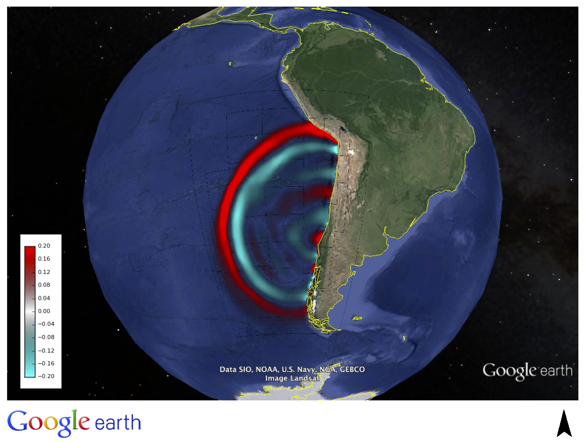
Simulation of the Chile 2010 tsunami (see geoclaw/examples/tsunami/chile2010).
Plotting attributes needed for Google Earth
The plotting parameters needed to instruct VisClaw to create plots suitable for visualization in Google Earth are all set as attributes of instances of the VisClaw classes ClawPlotData and ClawPlotFigure. We describe each of the relevant attributes and refer to their usage in the Chile 2010 example file setplot_kml.py file.
In what follows, we only refer to instances plotdata and plotfigure of the ClawPlotData and ClawPlotFigure classes.
plotdata attributes
The following plotdata attributes apply to all VisClaw figures to be visualized in Google Earth. These attributes are all optional and have reasonable default values.
#-----------------------------------------
# plotdata attributes for KML
#-----------------------------------------
plotdata.kml_name = "Chile 2010"
plotdata.kml_starttime = [2010,2,27,6,34,0]  # Date and time of event in UTC [None]
plotdata.kml_tz_offset = 3    # Time zone offset (in hours) of event. [None]

plotdata.kml_index_fname = "Chile_2010"  # name for .kmz and .kml files ["_GoogleEarth"]

plotdata.kml_user_files.append(['Santiago.kml',True])  # Extra user defined file.

# Set to a URL where KMZ file will be published.
# plotdata.kml_publish = None

# plotdata.kml_map_topo_to_latlong = None  # Use if topo coords. are not lat/long [None]
- kml_name : string
Name used in the Google Earth sidebar to identify the simulation. Default : “GeoClaw”
- kml_starttime : [Y,M,D,H,M,S]
Start date and time, in UTC, of the event. The format is [year,month,day,hour, minute, second]. By default, local time will be used.
- kml_timezone : integer
Time zone offset, in hours, of the event from UTC. For example, the offset for Chile is +3 hours, whereas the offset for Japan is -9 hours. Default : no time zone offset.
- kml_index_fname : string
The name given to the KMZ file created in the plot directory. Default : “_GoogleEarth”
- kml_publish : string
A URL address and path to a remote site hosting a KMZ file you wish to make available on-line. Default : None
See Publishing your results for more details.
- kml_map_topo_to_latlong : function
A function that maps computational coordinates (in meters, for example) to latitude/longitude coordinates. This will be called to position PNG overlays, gauges, patch boundaries, and regions boundaries to the latitude longitude box specified in plotfigure.kml_xlimits and plotfigure.kml_ylimits used by Google Earth. Default : None.
See Mapping topography data to latitude/longitude coordinates for details on how to set this function.
- kml_use_figure_limits : boolean
Set to True to indicate that the plotfigure limits should be used as axes limits when creating the PNG file. If set to False, then axes limits set by an axes member of a plotfigure (e.g. plotaxes) will be used. Default : True.
- kml_user_files : list
A list of extra user KML files to be archived along with image files and other plotting artifacts created by the VisClaw GoogleEarth plotting routines. These user files can contain, for example, additional placemarks, polygons, paths or other geographic features of relevance to the simulation. These geographic features will be copied to the KMZ archive and viewable in GoogleEarth, along with the results of the GeoClaw simulation.
The additional files to be archived are assumed to exist in the working directory (i.e. the directory containing the plots and output directories). For each file to be included, append a list of the form [filename, visibility] where filename is the KML file name (with the .kml extension) and visibility is either True or False. Append this list to the plotdata attribute, as in the example above. Default : No user files are included.
plotfigure attributes
The following attributes apply to an individual figure created for visualization in Google Earth. The first three attributes are required. The remaining attributes are optional.
The name “Sea Surface” given to the new instance plotfigure, below, will be used in the Google Earth sidebar to identify this figure.
#-----------------------------------------------------------
# Figure - Sea Surface
#----------------------------------------------------------
plotfigure = plotdata.new_plotfigure(name='Sea Surface',figno=1)
plotfigure.show = True

# Required KML attributes for visualization in Google Earth
plotfigure.use_for_kml = True
plotfigure.kml_xlimits = [-120,-60]    # Longitude
plotfigure.kml_ylimits = [-60, 0.0]    # Latitude

# Optional attributes
plotfigure.kml_use_for_initial_view = True
plotfigure.kml_figsize = [30.0,30.0]
plotfigure.kml_dpi = 12         # Resolve all three levels
plotfigure.kml_tile_images = False    # Tile images for faster loading.  Requires GDAL [False]
- use_for_kml : boolean
Indicates to VisClaw that the PNG files created for this figure should be suitable for visualization in Google Earth. With this set to True, all titles, axes labels, colorbars and tick marks will be suppressed. Default : False.
- kml_xlimits : [longitude_min, longitude_max]
Longitude range used to place PNG images on Google Earth. This setting will override any limits set as plotaxes attributes. Required
- kml_ylimits : [latitude_min, latitude_max]
Latitude range used to place the PNG images on Google Earth. This setting will override any limits set as plotaxes attributes. Required
- kml_use_for_initial_view : boolean
Set to True if this figure should be used to determine the initial camera position in Google Earth. The initial camera position will be centered over this figure at an elevation equal to approximately twice the width of the figure, in meters. By default, the first figure encountered with the use_for_kml attribute set to True will be used to set the initial view.
- kml_figsize : [size_x_inches,size_y_inches]
The figure size, in inches, for the PNG file. See Removing aliasing artifacts for tips on how to set the figure size and dpi for best results. Default : 8 x 6 (chosen by Matplotlib).
- kml_dpi : integer
Number of pixels per inch used in rendering PNG figures. For best results, figure size and dpi should be set to respect the numerical resolution of the the simulation. See Removing aliasing artifacts below for more details on how to improve the quality of the PNG files created by Matplotlib. Default : 200.
- kml_tile_images : boolean
Set to True if you want to create a pyramid of images at different resolutions for faster loading in Google Earth. Image tiling requires the GDAL library. See Optional GDAL library, above, for installation instructions. Default : False.
Creating the figures
All figures created for Google Earth are rendered as PNG files using the Matplotlib backend. So in this sense, the resulting PNG files are created in a manner that is no different from other VisClaw output formats. Furthermore, there are no special plotaxes or plotitem attributes to set for KML figures. But several attributes will either be ignored by the KML output or should be suppressed for best results in Google Earth.
# Create the figure
plotaxes = plotfigure.new_plotaxes('kml')

# Create a pseudo-color plot.  Render the sea level height transparent.
plotitem = plotaxes.new_plotitem(plot_type='2d_pcolor')
plotitem.plot_var = geoplot.surface_or_depth
plotitem.cmin = -0.2
plotitem.cmap = 0.2
plotitem.pcolor_cmap = googleearth_transparent

# Create a colorbar (appears as a Screen Overlay in Google Earth).
def kml_colorbar(filename):
  cmin = -0.2
  cmax = 0.2
  cmap = geoplot.googleearth_transparent
  geoplot.kml_build_colorbar(filename,cmap,cmin,cmax)

plotfigure.kml_colorbar = kml_colorbar
plotaxes attributes
The plotaxes attributes colorbar, xlimits, ylimits and title will all be ignored by the KML plotting. For best results, the attribute scaled should be set to its default value False. The only plotaxes attribute that might be useful in some limited contexts is the afteraxes setting, and only if the afteraxes function does not add plot features that cause Matplotlib to alter the space occupied by the figure. In most cases, the afteraxes commands should not be needed or should not be used.
plotitem attributes
The most useful plotitem type will probably be the 2d_pcolor type, although other types including the filled contour contourf can also be used to good effect.
Colormaps that are designed to work well with Google Earth are
geoplot.googleearth_transparent
geoplot.googleearth_lightblue
geoplot.googleearth_darkblue
The transparent colormap is particularly appealing visually when overlaid onto the Google Earth because the ocean bathymetry is clearly visible, illustrating the effect that underwater ridges and so on have on the propagating tsunami. The other two colormaps are solid colormaps, where the sea level color is set to match that of lighter or darker regions of the Google Earth ocean bathymetry.
Adding a colorbar overlay
A colorbar can be associated with each figure in the Google Earth browser by setting the figure attribute kml_colorbar to point to a function that creates the colorbar:
# Create a colorbar (appears as a Screen Overlay in Google Earth).
def kml_colorbar(filename):
  cmin = -0.2
  cmax = 0.2
  cmap = geoplot.googleearth_transparent
  geoplot.kml_build_colorbar(filename,cmap,cmin,cmax)

plotfigure.kml_colorbar = kml_colorbar
The color axis range [cmin, cmax] and the colormap cmap should be consistent with those set as plotitem attributes. By expanding the figure folder in the Google Earth sidebar, you can use check boxes to hide or show the colorbar screen overlay.
The input argument filename should be passed unaltered to the routine geoplot.kml_build_colorbar.
Gauge plots
There are no particular attributes for gauge plots and so they can be created in the usual way. In the Google Earth browser, gauge locations will be displayed as Placemarks. Clicking on gauge Placemarks will bring up the individual gauge plots. The screenshot below shows the gauge plot that appears when either the gauge Placemark or the gauge label in the sidebar is clicked.
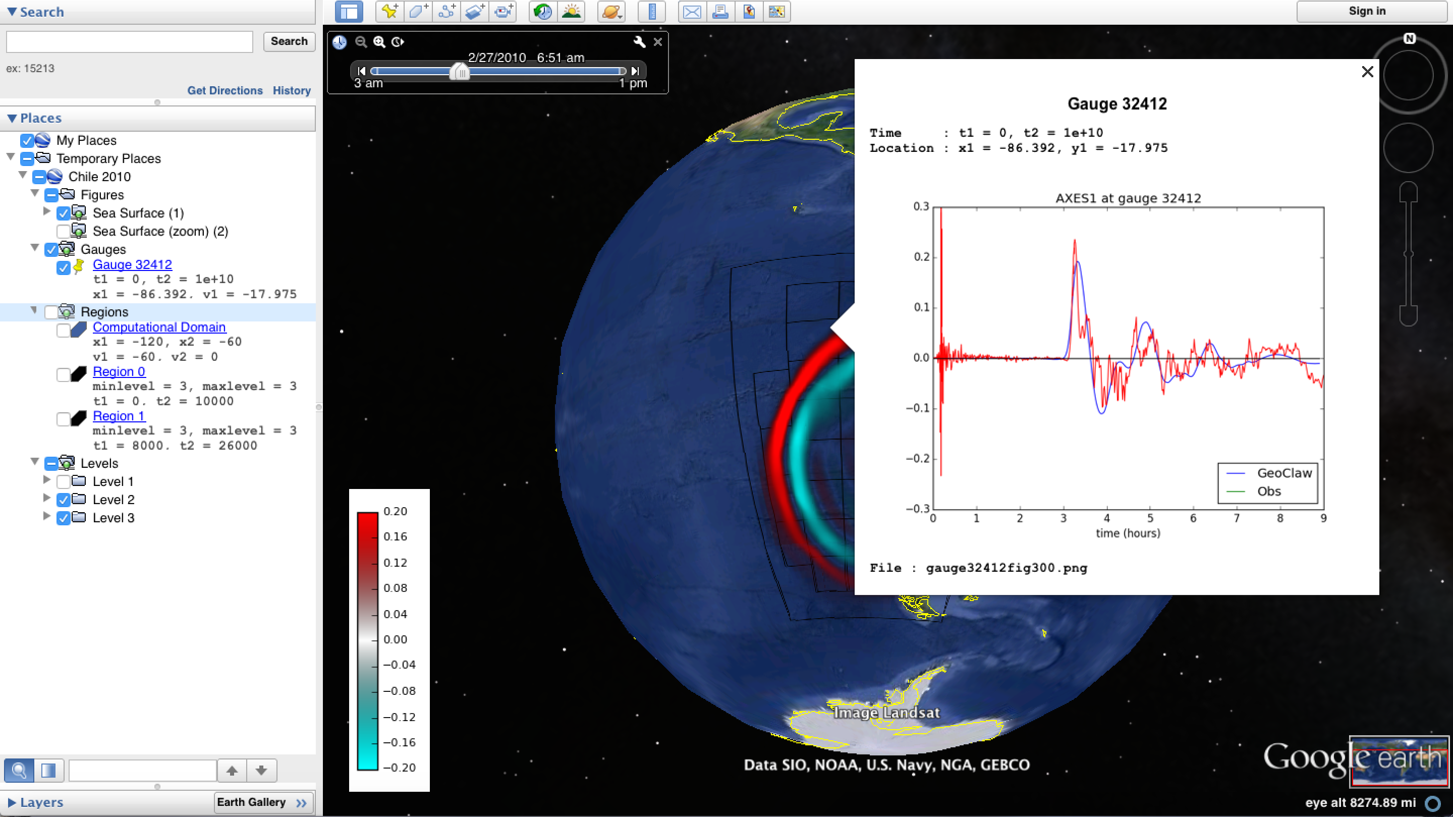
Screenshot illustrating gauge plots.
If the computational coordinates are not in latitude/longitude coordinates, then you must set the plotdata attribute map_topo_to_latlong to specify a mapping between the computational coordinates and latitude longitude box which Google Earth will use to visualize your data. See plotdata attributes.
Additional plotdata attributes
VisClaw has additional plotdata attributes indicating which figures and frames to plot and which output style to create. When plotting for Google Earth, one additional output parameter is necessary.
#-----------------------------------------
plotdata.print_format = 'png'      # file format
plotdata.print_framenos = 'all'    # list of frames to print
plotdata.print_fignos = 'all'      # list of figures to print
plotdata.html = False              # create html files of plots?
plotdata.latex = False             # create latex file of plots?
# ....
plotdata.kml = True        # <====== Set to True to create KML/KMZ output

return plotdata   # end of setplot_kml.py file
- kml : boolean
Set to True to indicate that a KML/KMZ file should be created. Default : False.
Plotting tips
Below are tips for working with KML/KMZ files, creating zoomed images, improving the quality of your images and publishing your results.
KML and KMZ files
KML files are very similar to HTML files in that they contan <tags>…</tags> describing data to be rendered by a suitable rendering engine. Whereas as standard web browsers can render content described by HTML tags, Google Earth renders the geospatial data described by KML-specific tags.
The kml attributes described above will direct VisClaw to create Google Earth suitable PNG files for frames and colorbars and a hierarchy of linked KML files, including a top level doc.kml file for the entire simulation, one top level doc.kml file per figure, and additional referenced kml files per frame. These KML and image files will not appear individually in your plots directory, but are archived into a single KMZ file that you can load in Google Earth.
If you would like to browse the individual images and KML files created by VisClaw, you can extract them from the KMZ file using an un-archiving utility. On OSX, for example, you can use unzip to extract one or more individual files from the KMZ file. Other useful zip utilities include zip (used to create the KMZ file initially) and zipinfo.
One reason you might wish to view the contents of an individual KMZ file is to inspect the PNG images generated by Matplotlib and used as GroundOverlays in the Google Earth browser. Another reason may be that you wish to make minor edits the top level doc.kml file to add additional Google Earth sidebar entries or to change visibility defaults of individual folders.
The KMZ file can be posted to a website to share your results with others. See Publishing your results, below.
Tiling images for faster loading
If you create several frames with relatively high dpi, you may find that the resulting KMZ file is slow to load in Google Earth. In extreme cases, large PNG files will not load at all. You can improve Google Earth performance by creating an image hierarchy which loads only a low resolution sampling of the data at low zoom levels and higher resolution images suitable for close-up views. In VisClaw, this image pyramid is created by setting the plotfigure attribute kml_tile_images to True.
plotfigure.kml_tile_images = True
Note: This requires the GDAL library, which can be installed following the Optional GDAL library instructions, above.
Removing aliasing artifacts
You may find that the transparent colormap leads to unappealing visual artifacts. This can happen when the resolution of the PNG file does not match the resolution of the data used to create the image. In the Chile example, the number of grid cells on the coarsest level is 30 in each direction. Two additional levels are created by refining first by a factor of 2 and then by a factor of 6. But the default settings for the figure size (kml_figsize) is 8x6 inches and dpi (kml_dpi) is 200, resulting in an image that is 1600 x 1200. But because 1600 is not an even multiple of 30, noticeable vertical stripes appear at the coarsest level. A more obvious plaid pattern appears at finer levels, since neither 1600 or 1200 are evenly divisible by 30*2*6 = 360.
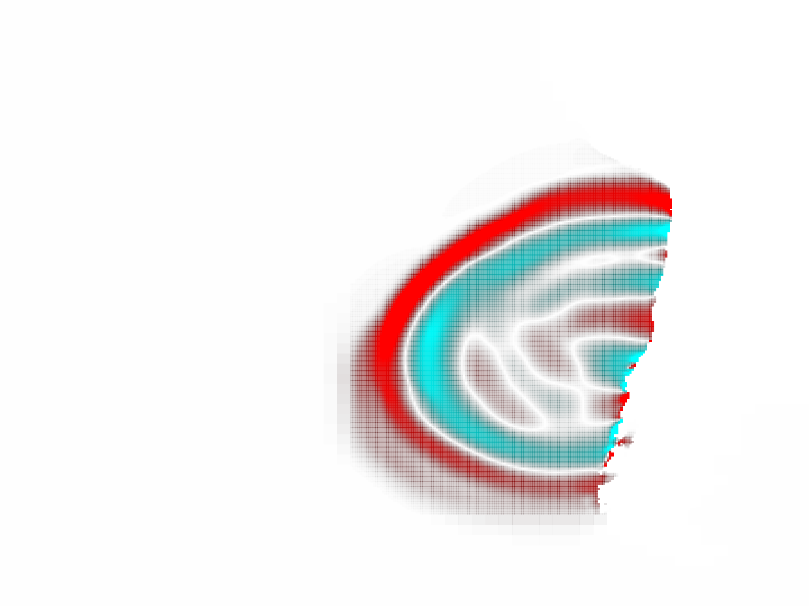
Aliasing effects resulting from default kml_dpi and kml_figsize settings
We can remove these aliasing effects by making the resolution of the PNG file a multiple of 30*2*6 = 360. This can be done by setting the figure size and dpi appropriately:
# Set dpi and figure size to resolve the 30x30 coarse grid, and two levels of refinement with
# refinement factors of 2 and 6.
plotfigure.kml_figsize = [30,30]
plotfigure.kml_dpi = 12
The resulting PNG file has a resolution of only 360x360, but in fact, is free of the vertical and horizontal stripes that appeared in the much higher resolution image created from the default settings.
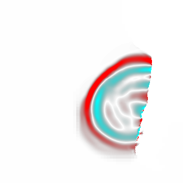
Aliasing effects removed by properly setting kml_dpi and kml_figsize
This baseline dpi=12 is the minimum resolution that will remove striped artifacts from your images. However, you may find that this resolution is unacceptable, especially for close-up views of shorelines and so on. In this case, you can increase the resolution of the figure by integer factors of the baseline dpi. In the Chile example, you might try increasing the dpi to 24 or even 48. The resulting PNG file, when rendered in Google Earth, should be much sharper when zoomed in for coastline views.
In some cases, it might not be possible to fully resolve all levels of a large multi-level simulation because the resulting image resolution would exceed the Matplotlib limit of 32768 pixels on a side. In this case, you can limit the number of levels that are resolved by a particular figure and create zoomed in figures to resolve finer levels. See Creating multiple figures at different resolutions, below. Alternatively, you can break the computational domain into several figures, each covering a portion of the entire domain.
If you set kml_dpi to a value less than 10, Matplotlib will revert to a dpi of 72 and change the figure size accordingly, so that the total number of pixels in each direction will still be equal to kml_figsize*kml_dpi, subject to round-off error. While you can avoid aliasing effects if this happens (assuming the dpi is still consistent with the resolution of the simulation), you can prevent Matplotlib from switching to a 72 dpi by simply reducing your figure size by a factor of 10 and increasing your dpi by a factor of 10.
Creating multiple figures at different resolutions
You can create several figures for visualization in Google Earth. Each figure you create will show up as a separate named folder in the Google Earth sidebar. The name will match that given to the VisClaw plotfigure.
For at least one figure, you will probably want to set the kml_xlimits and kml_ylimits to match the computational domain. To get higher resolution zoomed in figures, you will want to restrict the x- and y-limits to a smaller region. For best results, these zoom regions should be consistent with the resolution of your simulation. In the Chile example, a 30x30 inch figure resolves two degrees per inch. The x- and y-limits for the zoomed in figure should then span an even number of degrees in each direction, and have boundaries that align with even degree marks, i.e. -120, -118, -116, etc. In setplot_kml.py, the zoomed in region is described as :
#-----------------------------------------------------------
# Figure for KML files (zoom)
#----------------------------------------------------------
plotfigure = plotdata.new_plotfigure(name='Sea Surface (zoom)',figno=2)
plotfigure.show = True

plotfigure.use_for_kml = True
plotfigure.kml_use_for_initial_view = False  # Use large plot for view

# Zoomed figure created for Chile example.
plotfigure.kml_xlimits = [-84,-74]    # 10 degrees
plotfigure.kml_ylimits = [-18,-4]     # 14 degrees
plotfigure.kml_figsize = [10,14]  # inches. (1 inch per degree)

# Resolution
rcl = 10    # Over-resolve the coarsest level
plotfigure.kml_dpi = rcl*2*6       # Resolve all three levels
plotfigure.kml_tile_images = False  # Tile images for faster loading.
The resulting figure will have a resolution of 120 dots (i.e. pixels) per inch, compared to the 12 dpi in the larger PNG file covering the whole domain. The resolution of the zoomed image is 1200x1680, compared to 360x360 for the larger domain.
This higher resolution figure shows up in the Google Earth sidebar as “Sea Surface (zoom)”.
See Removing aliasing artifacts for more details on how to set the zoom levels.
Mapping topography data to latitude/longitude coordinates
In many situations, your computational domain may not be conveniently described in latitude/longitude coordinates. When simulating overland flooding events, for example, topographic data may more easily be described in rasterized distance increments (meters, for example). VisClaw uses data stored in generated data files (gauges.data, regions.data, and so on) to position objects on the Google Earth browser. The coordinate system for these objects is, however, in computational coordinates, and so to locate them in the Google Earth browser, the user must provide VisClaw a function to convert from computational to latitude/longtitude coordinates. This is done by setting the plotdata attribute kml_map_topo_to_latlong to a function describing your mapping between the two coordinate systems.
A crucial underlying assumption in setting the mapping function for use with GoogleEarth is that the boundary of your physical domain is approximately aligned with spherical (latitude/longitude) coordinate lines.
The following example illustrates how to set a linear map between the coordinates in [0,48000]x[0,17540] and the latitude/longitude coordinates that Google Earth will use to visualize the results of your simulation.
def map_cart_to_latlong(xc,yc):
    # Map x-coordinates
    topo_xlim = [0,48000]                     # x-limits, in meters
    ge_xlim = [-111.96132553, -111.36256443]  # longitude limits
    slope_x = (ge_xlim[1]-ge_xlim[0])/(topo_xlim[1]-topo_xlim[0])
    xp = slope_x*(xc-topo_xlim[0]) + ge_xlim[0]

    # Map y-coordinates
    topo_ylim = [0,17500]                     # y-limits, in meters
    ge_ylim = [43.79453362, 43.95123268]      # latitude limits
    slope_y = (ge_ylim[1]-ge_ylim[0])/(topo_ylim[1]-topo_ylim[0])
    yp = slope_y*(yc-topo_ylim[0]) + ge_ylim[0]

    return xp,yp

# set plotdata attribute.
plotdata.kml_map_topo_to_latlong = map_cart_to_latlong
Figure limits plotfigure.kml_xlimits and plotfigure.kml_ylimits must still be set to the latitude/longitude coordinates for your Google Earth figure. But to indicate that you do not wish to use these coordinates for creating PNG files, you must set the plotfigure.kml_use_figure_limits attribute to False. This will indicate that when creating the PNG figure, the axes limits should be set to those specifed in the plotaxes attribute. For example,
plotfigure = plotdata.new_plotfigure(name='Teton Dam',figno=1)
plotfigure.use_for_kml = True

# Latlong box used for GoogleEarth
plotfigure.kml_xlimits = [-111.96132553, -111.36256443]  #  Lat/Long box use by Google Earth
plotfigure.kml_ylimits = [43.79453362, 43.95123268]

# Use computational coordinates for plotting
plotfigure.kml_use_figure_limits = False   # Use plotaxes limits below

# ....

plotaxes.xlimits = [0,48000]   # Computational axes needed for creating PNG files.
plotaxes.ylimits = [0,17500]
The mapping function will be used to position PNG Overlays, locate gauge placemarks, and plot patch and region boundaries on the Google Earth browser.
Publishing your results
You can easily share your results with collaborators by providing links to your archive KMZ file in HTML webpages. Collaborators can download the KMZ file and open it in a Google Earth browser.
If you find that the KMZ file is too large to make downloading convenient, you can provide a light-weight KML file that contains a link to your KMZ file stored on a host server. Collaborators can then open this KML file in Google Earth and browse your results remotely.
VisClaw offers an option to automatically create a sample KML file containing a link to your KMZ file. To create this KML file, you should set the plotdata attribute kml_publish to the url address of your host server where the KMZ files will be stored. For example, the Chile file above is stored at:
plotdata.kml_publish = "http://math.boisestate.edu/~calhoun/visclaw/GoogleEarth/kmz"
VisClaw will detect that this plotdata attribute has been set and automatically create a KML file that refers to the linked file “Chile_2010.kmz”, stored at the above address. This KML file (see Chile_2010.kml for an example) can be easily edited, shared or posted on webpages to allow collaborators to view your results via links to your remotely stored KMZ file.
By default, plotdata.kml_publish is set to None, in which case, no KML file will be created.