Force Cells to be Dry Initially
New in Version 5.7.0.
Adapted from this notebook.
See also Marching Front algorithm, which describes a tool to select points from a topography DEM that satisfy given constraints on elevation, and how this can be used to determine dry land behind dikes.
This can then be used to define an array that can be read into GeoClaw and used when initializing the water depth during the creation of new grid patches. See the section Usage in GeoClaw Fortran code for instructions on how to specify this in setrun.py.
We define an rectangular array force_dry_init that is aligned with cell centers of the computational grid at some resolution (typically the finest resolution) and that has the value force_dry_init[i,j] = 1 to indicate cells that should be initialized to dry (h[i,j] = 0) regardless of the value of the GeoClaw topography B[i,j] in this cell. If force_dry_init[i,j] = 0 the the cell is initialized in the usual manner, which generally means
h[i,j] = max(0, sea_level - B[i,j]).
Notes:
Another new feature allows initializing the depth so that the surface elevation eta is spatially varying rather than using a single scalar value sea_level everywhere. That feature is described in Set Eta Init – spatially varying initial surface elevation. If that is used in conjunction with a force_dry_init array, force_dry_init[i,j] = 1 still indicates that the cell should be dry while elsewhere the “usual” thing is done.
The current implementation allows only one force_dry_init array but in the future this may be generalized to allow multiple arrays covering different subsets of the domain, and perhaps at different grid resolutions.
Typically the force_dry_init array is computed from a DEM file at the desired resolution, using the marching front algorithm defined in Marching Front algorithm. But recall that the GeoClaw topography value B[i,j] does not agree with the DEM value Z[i,j] even if the cell center is aligned with the DEM point due to the way B is computed by averaging over piecewise bilinear functions that interpolate the Z values. So one has to be careful not to set force_dry_init[i,j] = 1 in a cell close to the shore simply because Z > 0 at this point since the B value might be negative in the cell. This is dealt with in the examples below by doing some buffering.
Contents
Examples
First import some needed modules and set up color maps.
%matplotlib inline
from pylab import *
import os,sys
from numpy import ma # masked arrays
from clawpack.visclaw import colormaps

from clawpack.geoclaw import marching_front, topotools
from clawpack.amrclaw import region_tools
from clawpack.visclaw import plottools
zmin = -60.
zmax = 40.

land_cmap = colormaps.make_colormap({ 0.0:[0.1,0.4,0.0],
                                     0.25:[0.0,1.0,0.0],
                                      0.5:[0.8,1.0,0.5],
                                      1.0:[0.8,0.5,0.2]})

sea_cmap = colormaps.make_colormap({ 0.0:[0,0,1], 1.:[.8,.8,1]})

cmap, norm = colormaps.add_colormaps((land_cmap, sea_cmap),
                                     data_limits=(zmin,zmax),
                                     data_break=0.)

sea_cmap_dry = colormaps.make_colormap({ 0.0:[1.0,0.7,0.7], 1.:[1.0,0.7,0.7]})
cmap_dry, norm_dry = colormaps.add_colormaps((land_cmap, sea_cmap_dry),
                                     data_limits=(zmin,zmax),
                                     data_break=0.)
Sample topography from a 1/3 arcsecond DEM
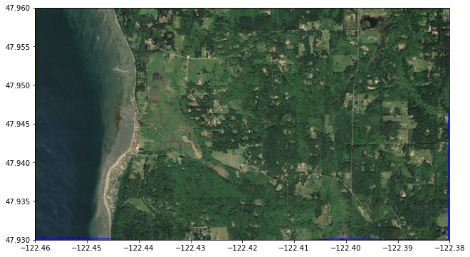
We consider a small region on the SW coast of Whidbey Island north of Maxwelton Beach as an example, as was used in MarchingFront.ipynb.
region1_png = imread('region1.png')
extent = [-122.46, -122.38, 47.93, 47.96]

figure(figsize=(12,6))
imshow(region1_png, extent=extent)
gca().set_aspect(1./cos(48*pi/180.))
We read this small portion of the 1/3 arcsecond Puget Sound DEM, available from the NCEI thredds server:
path = 'https://www.ngdc.noaa.gov/thredds/dodsC/regional/puget_sound_13_mhw_2014.nc'
topo = topotools.read_netcdf(path, extent=extent)
Plot the topo we downloaded:
figure(figsize=(12,6))
plottools.pcolorcells(topo.X, topo.Y, topo.Z, cmap=cmap, norm=norm)
colorbar(extend='both')
gca().set_aspect(1./cos(48*pi/180.))
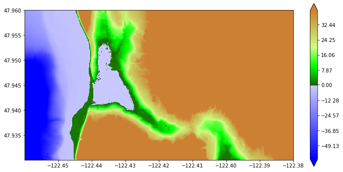
This plot shows that there is a region with elevation below MHW (0 in the DEM) where the Google Earth image shows wetland that should not be initialized as a lake. We repeat the code used in Marching Front algorithm to identify dry land below MHW:
wet_points = marching_front.select_by_flooding(topo.Z, Z1=-5., Z2=0., max_iters=None)

Zdry = ma.masked_array(topo.Z, wet_points)

figure(figsize=(12,6))
plottools.pcolorcells(topo.X, topo.Y, Zdry, cmap=cmap, norm=norm)
colorbar(extend='both')
gca().set_aspect(1./cos(48*pi/180.))
title('Dry land');
Selecting points with Z1 = -5, Z2 = 0, max_iters=279936
Done after 112 iterations with 59775 points chosen
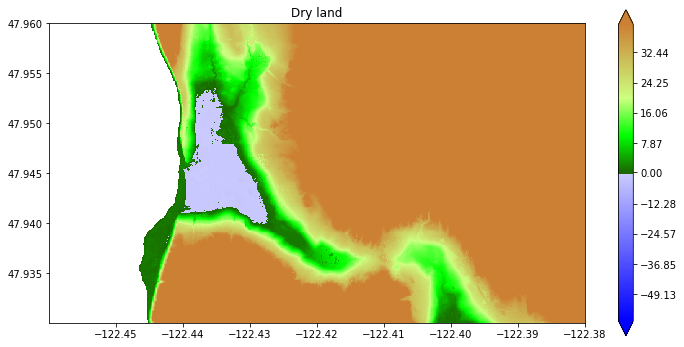
Now the blue region above is properly identified as being dry land.
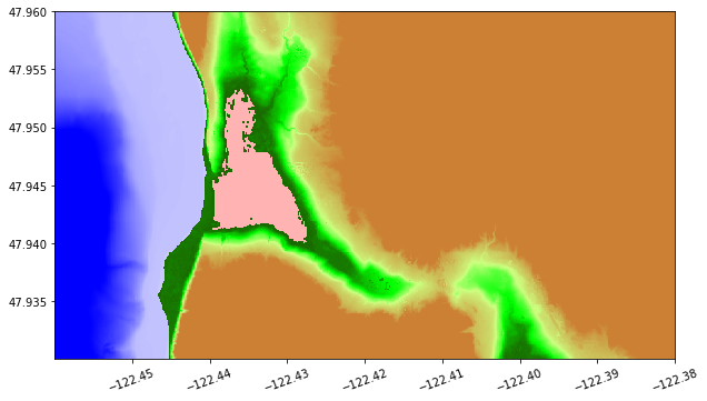
The colors are misleading, so here’s a way to plot with the dry land that is below MHW colored pink to distinguish it from the water better:
# Create a version of topo.Z with all wet points masked out:
mask_dry = logical_not(wet_points)
Z_dry = ma.masked_array(topo.Z, wet_points)

# Create a version of topo.Z with only dry points below MHW masked out:
mask_dry_onshore = logical_and(mask_dry, topo.Z<0.)
Z_allow_wet= ma.masked_array(topo.Z, mask_dry_onshore)

figure(figsize=(10,12))

# first plot all dry points as pink:
plottools.pcolorcells(topo.X, topo.Y, Z_dry, cmap=cmap_dry, norm=norm_dry)

# then plot colored by topography except at dry points below MHW:
plottools.pcolorcells(topo.X, topo.Y, Z_allow_wet, cmap=cmap, norm=norm)

gca().set_aspect(1./cos(48*pi/180.))
ticklabel_format(useOffset=False)
xticks(rotation=20);
Creating the force_dry_init array
The array wet_points generated above has the value 1 at DEM points identified as wet and 0 at points identified as dry, so if we set
dry_points = 1 - wet_points
then dry_points[i,j] = 1 at the DEM points determined to be dry. We do not necessarily want to force the GeoClaw cell to be dry however at all these dry points, because the GeoClaw topography value B may be slightly negative even if the DEM value Z was positive at the same point, due to the way B is computed, and so this might force some cells near the shore to have h = 0 even though B < 0.
Instead we will set force_dry_init[i,j] = 1 only if dry_points[i,j] = 1 and the same is true of all its 8 nearest neighbors. This avoids problems near the proper shoreline while forcing cells inland to be dry where they should be.
We also assume it is fine to set force_dry_init[i,j] = 0 around the boundary of the grid on which dry_points has been defined, so that the usual GeoClaw procedure is used to initialize these points. If there are points at the boundary that must be forced to be dry that we should have started with a large grid patch.
So we can accomplish this by summing the dry_points array over 3x3 blocks and setting force_dry_init[i,j] = 1 only at points where this sum is 9:
dry_points_sum = dry_points[1:-1,1:-1] + dry_points[0:-2,1:-1] + dry_points[2:,1:-1] + \
                 dry_points[1:-1,0:-2] + dry_points[0:-2,0:-2] + dry_points[2:,0:-2] + \
                 dry_points[1:-1,2:] + dry_points[0:-2,2:] + dry_points[2:,2:]

# initialize array to 0 everywhere:
force_dry_init = zeros(dry_points.shape)
# reset in interior to 1 if all points in the 3x3 block around it are dry:
force_dry_init[1:-1,1:-1] = where(dry_points_sum == 9, 1, 0)
If we use 1-force_dry_init as a mask then we see only the points forced to be dry:
Zdry = ma.masked_array(topo.Z, 1-force_dry_init)

figure(figsize=(12,6))
plottools.pcolorcells(topo.X, topo.Y, Zdry, cmap=cmap, norm=norm)
colorbar(extend='both')
gca().set_aspect(1./cos(48*pi/180.))
title('Points with force_dry_init==1')
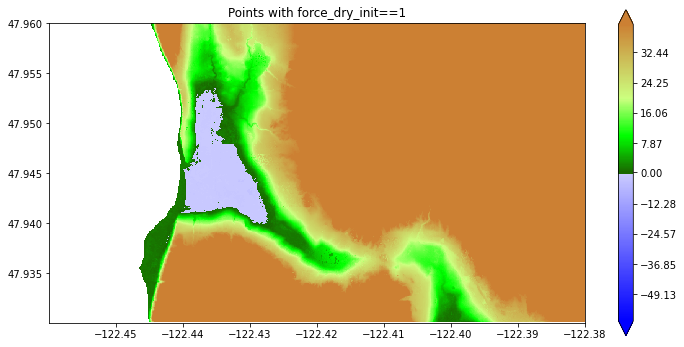
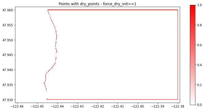
This looks a lot like the plot above where we masked with wet_points. However, if we plot dry_points - force_dry_init we see that this is not identically zero – and there are points along the shore and the boundaries where the point was identified as dry but will not be forced to be dry:
figure(figsize=(12,6))
plottools.pcolorcells(topo.X, topo.Y, dry_points - force_dry_init,
                      cmap=colormaps.white_red)
colorbar()
gca().set_aspect(1./cos(48*pi/180.))
axis([-122.461, -122.379, 47.929, 47.961]) # expanded domain
title('Points with dry_points - force_dry_init==1');
Create file to read into GeoClaw
The array force_dry_init can now be saved in the same format as topo files, using topo_type=3 and specifying Z_format=’%1i’ so that the data values from the array, which are all either 0 or 1, are printed as single digits to help reduce the file size.
Note we also use the new convenience fuction set_xyZ introduced in topotools.Topography.
force_dry_init_topo = topotools.Topography()
force_dry_init_topo.set_xyZ(topo.x, topo.y, force_dry_init)

# Old way of setting x,y,Z:
#force_dry_init_topo._x = topo.x
#force_dry_init_topo._y = topo.y
#force_dry_init_topo._Z = force_dry_init
#force_dry_init_topo.generate_2d_coordinates()

fname_force_dry_init = 'force_dry_init.data'
force_dry_init_topo.write(fname_force_dry_init, topo_type=3, Z_format='%1i')
print('Created %s' % fname_force_dry_init)
Created force_dry_init.data
As usual, the first 6 lines of this file are the header, which is then followed by the data:
864                              ncols
324                              nrows
-1.224599074275750e+02              xlower
4.793009258334999e+01              ylower
9.259259000800000e-05              cellsize
-9999                          nodata_value
Usage in GeoClaw Fortran code
To use a force_dry_init.data file of the sort created above, when setting up a GeoClaw run the setrun.py file must be modified to indicate the name of this file along with a time tend. The array is used when initializing new grid patches only if t < tend, so this time should be set to a time after the finest grids are initialized, but before the tsunami arrives.
For example, to use the file force_dry_init.data to indicate cells that should be forced to be dry for times up to 15 minutes, we could specify:
from clawpack.geoclaw.data import ForceDry
force_dry = ForceDry()
force_dry.tend = 15*60.
force_dry.fname = 'force_dry_init.data'
rundata.qinit_data.force_dry_list.append(force_dry)
Internal GeoClaw modifications
The following files in geoclaw/src/2d/shallow have been modified to handle the force_dry_init array:
setprob.f90 to read in a parameter indicating that there is such an array,
qinit_module.f90 with code to read the array,
qinit.f90 to initialize dry land properly at the initial time,
filpatch.f90 to initialize new grid patches properly at later times,
filval.f90 to initialize new grid patches properly at later times.
The force_dry_init array is used when initializing new patches only if:
The resolution of the patch agrees with that of the force_dry_init array, and it is then assumed that the points in the array are aligned with cell centers on the patch.
The simulation time t is less than t_stays_dry, a time set to be after the relevant level is introduced in the region of interest but before the main tsunami wave has arrived. At later times the tsunami may have gotten a region wet even if force_dry_init indicates is should be initially dry.