Marching Front algorithm
New in Version 5.7.0.
Adapted from this notebook.
The module clawpack.geoclaw.marching_front defines a function select_by_flooding that takes as input an array Ztopo containing topography elevations on a rectangular grid and returns an array pt_chosen of the same shape with values 1 (if chosen) or 0 (if not chosen). Other inputs specify the criteria used to choose points, as described below.
The basic idea is that chosen points satisfy certain elevation requirements along with connectivity to the coast. This was originally developed to identify points in a topography DEM where the topography value \(Z\) is below MHW, but that should be initialized as dry land because they are in regions protected by dikes or levies. In this situation, the marching algorithm is used by initializing points well offshore (e.g. with \(Z < -5\) meters) as wet and other points to unset. Then the front between wet/unset points is advanced by marking neighboring points as dry if \(Z\geq0\) or as wet if \(Z<0\). This is repeated iteratively for each new front until there are no more wet points with unset neighbors. At this point any points still unset are entirely buffered by dry points and must lie behind dikes, so these are also set to dry.
The use of such a force_dry_array in GeoClaw is explained in Force Cells to be Dry Initially.
Other applications are also described below along with some examples.
Contents
Function arguments
The main function in the marching_front.py module is select_by_flooding.
The function is defined by:
def select_by_flooding(Ztopo, mask=None, prev_pts_chosen=None,
                       Z1=-5., Z2=0., max_iters=None, verbose=False):
If Z1 <= Z2 then points where Ztopo < Z1 are first selected and then a marching algorithm is used to select neighboring points that satisfy Ztopo < Z2.
Think of chosen points as “wet” and unchosen points as “dry” and new points are flooded if at least one neighbor is “wet” and the topography is low enough. Starting from deep water (e.g. Z1 = -5) this allows flooding up to MHW (Z2 = 0) without going past dikes that protect dry land with lower elevation.
However, this can also be called with Z1 > Z2, in which case points where Ztopo >= Z1 are first selected and then the marching algorithm is used to select neighboring points that satisfy Ztopo > Z2. This is useful to select offshore points where the water is shallow, (and that are connected to the shore by a path of shallow points) e.g. to identify points on the continental shelf to set up a flag region for refinement.
If max_iters=None then iterate to convergence. Otherwise, at most max_iters iterations are taken, so setting this to a small value only selects points within this many grid points of where Ztopo <= Z1, useful for buffering or selecting a few onshore points along the coast regardless of elevation.
If prev_pts_chosen is None we are starting from scratch, otherwise we possibly add additional chosen points to an existing array. Points where prev_pts_chosen[i,j]==1 won’t change but those ==0 may be changed to 1 based on the new criteria.
If mask==None or mask==False then the entire array is subject to selection. If mask is an array with mask[i,j]==True at some points, then either: - these masked points are marked as not selected (pts_chosen[i,j]=0) if prev_pts_chosen==None, or - these masked points are not touched if prev_pts_chosen is an array (so previous 0/1 values are preserved).
These arguments are described in more detail below with examples of how they might be used.
output array
The function returns an array pt_chosen with the same shape as Ztopo and has the value 1 at points chosen and 0 at points not chosen.
creating a masked array
This array can be used to define a masked array from Ztopo that masks out the points not chosen via:
from numpy import ma # masked array module
Zmasked = ma.masked_array(Ztopo, mask=logical_not(pt_chosen))
This could be used to plot only the points chosen using the matplotlib function pcolormesh, for example, or the function now defined in geoclaw.visclaw.plottools.pcolorcells that better plots finite volume grid cell data with proper alignment and boundary cells. See pcolorcells.
topofile mask for initializing dry points
The array pt_chosen can be used to create a file that is read in by GeoClaw to identify points where Ztopo is below MHW but where there is dry land because of protection by dikes or levies. This is done by defining a geoclaw.topotools.Topography object and setting its Z attribute based on pt_chosen, and then writing this as a topofile with topo_type==3. Then in setrun.py this file can be specified as a mask that is read in and used when initializing grid cells. There are some subtleties in how this is done, described in more detail in Force Cells to be Dry Initially.
fgmax points
The chosen points might be used as fgmax points, as described below.
flag regions
The output array could also be used to define an AMR flag region as a ruled rectangle, using the function region_tools.ruledrectangle_covering_selected_points described in Ruled Rectangles. This would give a minimal ruled rectangle covering all the chosen points. An example is given below.
The mask argument
mask can be False or None, or else must be an array of the same shape as Ztopo.
The Ztopo array input must be a rectangular array, but sometimes we want to select points covering only a subset of these points, e.g. when defining fgmax points along some stretch of coastline. In this case mask can be used to mask out values we do not want to select. Set mask[i,j] = True at points that should not be chosen.
To mask out points that lie outside some ruled rectangle that has been defined as rr, you can use the rr.mask_outside function to define the mask. See Ruled Rectangles.
The previous_pts_chosen argument
This argument is useful if you want to apply a sequence of different criteria to choose points. For example, suppose you first want to choose all grid points within 5 points of the coast (as can be done using max_iters) and then supplement this will all grid points below a specified elevation that are farther inland from the coast.
Examples are given below, also of how the mask array works in conjunction with previous_pts_chosen.
Examples
First import some needed modules and set up color maps.
import os,sys
from numpy import ma # masked arrays
from clawpack.visclaw import colormaps
from clawpack.geoclaw import topotools, marching_front
from clawpack.amrclaw import region_tools
from clawpack.visclaw.plottools import pcolorcells

zmin = -60.
zmax = 40.

cmap_land = colormaps.make_colormap({ 0.0:[0.1,0.4,0.0],
                                     0.25:[0.0,1.0,0.0],
                                      0.5:[0.8,1.0,0.5],
                                      1.0:[0.8,0.5,0.2]})

cmap_sea = colormaps.make_colormap({ 0.0:[0,0,1], 1.:[.8,.8,1]})

cmap_topo, norm_topo = colormaps.add_colormaps((cmap_land, cmap_sea),
                                     data_limits=(zmin,zmax),
                                     data_break=0.)

cmap_sea_dry = colormaps.make_colormap({ 0.0:[1.0,0.7,0.7], 1.:[1.0,0.7,0.7]})
cmap_dry, norm_dry = colormaps.add_colormaps((cmap_land, cmap_sea_dry),
                                     data_limits=(zmin,zmax),
                                     data_break=0.)
Sample topography from a 1/3 arcsecond DEM
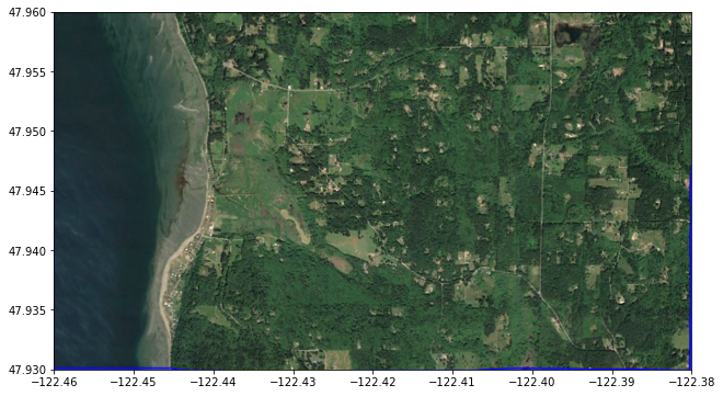
We consider a small region on the SW coast of Whidbey Island north of Maxwelton Beach as an example:
region1_png = imread('region1.png')
extent = [-122.46, -122.38, 47.93, 47.96]

figure(figsize=(12,6))
imshow(region1_png, extent=extent)
gca().set_aspect(1./cos(48*pi/180.))
We read this small portion of the 1/3 arcsecond Puget Sound DEM, available from the NCEI thredds server:
path = 'https://www.ngdc.noaa.gov/thredds/dodsC/regional/puget_sound_13_mhw_2014.nc'
topo = topotools.read_netcdf(path, extent=extent)
figure(figsize=(12,6))
pcolorcells(topo.X, topo.Y, topo.Z, cmap=cmap, norm=norm)
colorbar(extend='both')
gca().set_aspect(1./cos(48*pi/180.))

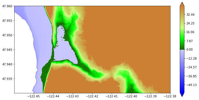
This plot shows that there is a region with elevation below MHW (0 in the DEM) where the Google Earth image shows wetland that should not be initialized as a lake. This problem is discussed in Force Cells to be Dry Initially.
Here we show how to choose only the DEM points that are close to the shore and/or below a given elevation.
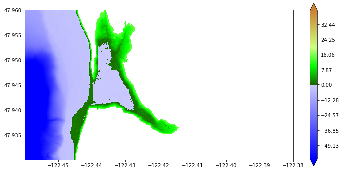
Finding all points below a given elevation
First we choose all points with elevation below 15 m and that are connected to the coast over this topography extent. Note the latter requirement will eliminate the low lying area at the bottom of the figure above near longitude -122.4 (which is connected to the coast through Cultus Bay, but not by points in this extent).
pts_chosen = marching_front.select_by_flooding(topo.Z, Z1=0, Z2=15., max_iters=None)
Selecting points with Z1 = 0, Z2 = 15, max_iters=279936
Done after 183 iterations with 89871 points chosen
Zmasked = ma.masked_array(topo.Z, logical_not(pts_chosen))

figure(figsize=(12,6))
pcolorcells(topo.X, topo.Y, Zmasked, cmap=cmap, norm=norm)
colorbar(extend='both')
gca().set_aspect(1./cos(48*pi/180.))
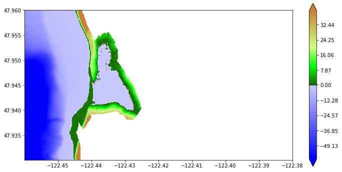
Create a buffer zone along shore
To select more points along the shore where the topography is steep, we could have first used max_iters.
To illustrate this, we start again and fist use max_iters = 20 so that at least 20 grid points are selected near the coast, also setting Z2 = 1e6 (a huge value) so that the arbitrarily high regions will be included if they are within 20 points of the coast:
pts_chosen = marching_front.select_by_flooding(topo.Z, Z1=0, Z2=1e6, max_iters=20)
Selecting points with Z1 = 0, Z2 = 1e+06, max_iters=20
Done after 20 iterations with 84800 points chosen
Plot what we have so far:
Zmasked = ma.masked_array(topo.Z, logical_not(pts_chosen))

figure(figsize=(12,6))
pcolorcells(topo.X, topo.Y, Zmasked, cmap=cmap, norm=norm)
colorbar(extend='both')
gca().set_aspect(1./cos(48*pi/180.))
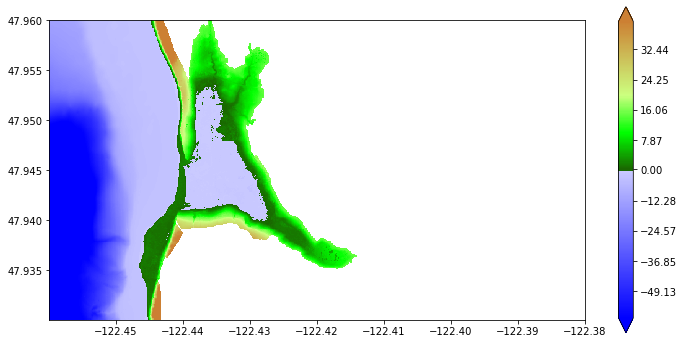
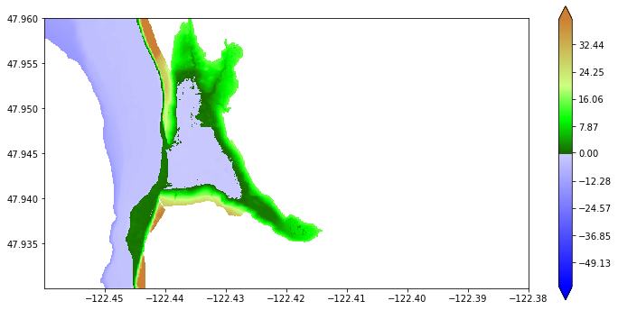
Then we augment the points already chosen with any points below 15 m and connected to the coast:
pts_chosen = marching_front.select_by_flooding(topo.Z, Z1=0, Z2=15.,
                                               prev_pts_chosen=pts_chosen,
                                               max_iters=None)
Selecting points with Z1 = 0, Z2 = 15, max_iters=279936
Done after 163 iterations with 94297 points chosen
Zmasked = ma.masked_array(topo.Z, logical_not(pts_chosen))

figure(figsize=(12,6))
pcolorcells(topo.X, topo.Y, Zmasked, cmap=cmap, norm=norm)
colorbar(extend='both')
gca().set_aspect(1./cos(48*pi/180.))
Choose points only near shore
We can set Z1 = 0 and Z2 = -15 to select points that have elevation greater than -15 m and are connected to the coast:
pts_chosen_shallow = marching_front.select_by_flooding(topo.Z, Z1=0, Z2=-15., max_iters=None)
Selecting points with Z1 = 0, Z2 = -15, max_iters=279936
Done after 177 iterations with 249577 points chosen
Zshallow = ma.masked_array(topo.Z, logical_not(pts_chosen_shallow))

figure(figsize=(12,6))
pcolorcells(topo.X, topo.Y, Zshallow, cmap=cmap, norm=norm)
colorbar(extend='both')
gca().set_aspect(1./cos(48*pi/180.))
Note that this chooses all onshore points in addition to offshore points with elevation greater than -15 m.
We can take the intersection of this set of points with the onshore points previously chosen to get only the points that lie near the coast:
pts_chosen_nearshore = logical_and(pts_chosen, pts_chosen_shallow)
Znearshore = ma.masked_array(topo.Z, logical_not(pts_chosen_nearshore))

figure(figsize=(12,6))
pcolorcells(topo.X, topo.Y, Znearshore, cmap=cmap, norm=norm)
colorbar(extend='both')
gca().set_aspect(1./cos(48*pi/180.))
Write out the masked array indicating fgmax points
One we have selected the desired fgmax points, these can be output in the style of a topo_type=3 topography file, with a header followed point values at all points on a uniform grid. The values are simply the integer 1 for points that should be used as fgmax points and 0 for other points. Note that format %1i is used for compactness.
fname_fgmax_mask = 'fgmax_pts_topostyle.data'
topo_fgmax_mask = topotools.Topography()
topo_fgmax_mask._x = topo.x
topo_fgmax_mask._y = topo.y
topo_fgmax_mask._Z = where(pts_chosen_nearshore, 1, 0)  # change boolean to 1/0
topo_fgmax_mask.generate_2d_coordinates()

topo_fgmax_mask.write(fname_fgmax_mask, topo_type=3, Z_format='%1i')
print('Created %s' % fname_fgmax_mask)
Created fgmax_pts_topostyle.data
This file fgmax_pts_topostyle.data can then be read into GeoClaw, using the new capability of specifying fgmax grids in this manner, using point_style == 4 as described in Fixed grid monitoring (fgmax).
Creating an AMR flag region
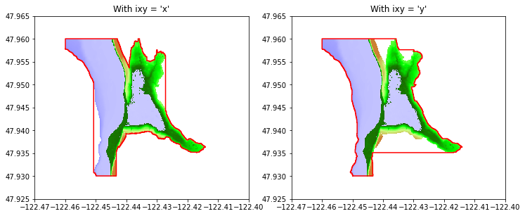
Once a set of points has been selected, it can be used to define a ruled rectangle that might be used as an adaptive mesh refinement flag region, for example. See Ruled Rectangles and Specifying flagregions for adaptive refinement.
You might want to try both ixy = ‘x’ and ixy = ‘y’ in creating the ruled rectangle to see which one covers fewer non-selected points. In this case ixy = ‘x’ is better:
figure(figsize=(12,5))
subplot(121)

rr = region_tools.ruledrectangle_covering_selected_points(topo.X, topo.Y, pts_chosen_nearshore,
                                                          ixy='x', method=0,
                                                          padding=0, verbose=True)
xv,yv = rr.vertices()
pcolorcells(topo.X, topo.Y, Znearshore, cmap=cmap, norm=norm)
axis([-122.47, -122.40, 47.925, 47.965])
gca().set_aspect(1./cos(48*pi/180.))
plot(xv, yv, 'r')
title("With ixy = 'x'")

subplot(122)
rr = region_tools.ruledrectangle_covering_selected_points(topo.X, topo.Y, pts_chosen_nearshore,
                                                          ixy='y', method=0,
                                                          padding=0, verbose=True)
xv,yv = rr.vertices()
pcolorcells(topo.X, topo.Y, Znearshore, cmap=cmap, norm=norm)
axis([-122.47, -122.40, 47.925, 47.965])
gca().set_aspect(1./cos(48*pi/180.))
plot(xv, yv, 'r')
title("With ixy = 'y'")
Extending rectangles to cover grid cells
RuledRectangle covers 69788 grid points
Extending rectangles to cover grid cells
RuledRectangle covers 76005 grid points
Determining dry areas below MHW
Note the blue region in the above plot that is inland from the coast and behind a green barrier. Examining Google Earth shows that this is wetland area that probably should not be initialized as a lake. We can identify this by using the marching front algorithm to start at Z1 = -5 m and fill in up to Z2 = 0 (MHW).
wet_points = marching_front.select_by_flooding(topo.Z, Z1=-5., Z2=0., max_iters=None)
Selecting points with Z1 = -5, Z2 = 0, max_iters=279936
Done after 112 iterations with 59775 points chosen
Zdry = ma.masked_array(topo.Z, wet_points)

figure(figsize=(12,6))
pcolorcells(topo.X, topo.Y, Zdry, cmap=cmap, norm=norm)
colorbar(extend='both')
gca().set_aspect(1./cos(48*pi/180.))
title('Dry land');
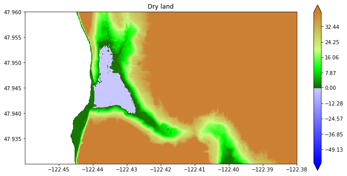
Now the blue region above is properly identified as being dry land.
See Force Cells to be Dry Initially for more discussion of this example, showing how to create an array for GeoClaw in order to indicate that this region should be initialized as dry in spite of being below MHW.