Ruled Rectangles
New in Version 5.7.0.
Adapted from this notebook.
In past versions of AMRClaw and GeoClaw, one could specify “refinement regions” as rectangles over which a minlevel and maxlevel are specified (perhaps over some time interval), as described in refinement-regions.
Allowing only rectangles made it very easy to check each cell for inclusion in a region, but is a severe restriction – often a number of rectangles must be used to follow a complicated coastline, for example, or else many points ended up being refined that did not require it (e.g. onshore points that never get wet in a GeoClaw simulation).
We have introduced a new data structure called a “Ruled Rectangle” that is a special type of polygon for which it is also easy to check whether a given point is inside or outside, but that is much more flexible than a rectangle. It is a special case of a “ruled surface”, which is a surface in 3D that is bounded by two curves, each parameterized by \(s\) from \(s_1\) to \(s_2\), and with the surface defined as the union of all the line segments connecting one curve to the other for each value of \(s\) in \([s_1,s_2]\). A Ruled Rectangle is a special case in which each curve lies in the \(x\)-\(y\) plane and either \(s=x\) for some range of \(x\) values or \(s=y\) for some range of \(y\) values. If \(s=x\), for example, then the line segments defining the surface are intervals \(y_{\scriptstyle lower}(x) \leq y \leq y_{\scriptstyle upper}(x)\) for each \(x\) over some range \(x_1 \leq x \leq x_2\). It is easy to check if a given \((x_c,y_c)\) is in this region: it is if \(x_1 \leq x_c \leq x_2\) and in addition \(y_{\scriptstyle lower}(x_c) \leq y_c \leq y_{\scriptstyle upper}(x_c)\).
The class clawpack.amrclaw.region_tools.RuledRectangle supports
a subset of ruled rectangles defined by a finite set of \(s\)
values along a coordinate line, e.g. \(s[0] < s[1] < s[2] <
\cdots < s[N]\) and for each \(s[k]\) two values lower[k] and
upper[k]. If rr is an instance of this class then rr.s,
rr.lower, and rr.upper contain these arrays. Whether s
corresponds to x or y is determined by:
If rr.ixy in [1, ‘x’] then s gives a set of \(x\) values,
If rr.ixy in [2, ‘y’] then s gives a set of \(y\) values.
The points specified can then be connected by line segments to define a Ruled Rectangle, and this is done if rr.method == 1 (piecewise linear). On the other hand, if rr.method == 0 (piecewise constant) then the values lower[k], upper[k] are used as the bounds for all s in the interval \(s[k] \leq s \leq s[k+1]\) (for \(k = 0,~1,~\ldots,~N-1\)). In this case the values lower[N], upper[N] are not used. This also defines a polygon, but one that consists of a set of stacked boxes. The advantage of the latter form is that it is slightly easier to check if a point is in the Ruled Rectangle since no linear interpolation is required along the edges. Also for some applications we want the Ruled Rectangle to exactly cover a contiguous set of finite volume grid cells, which has the shape of a set of stacked boxes.
Contents
Examples
Some simple examples follow:
Define a Ruled Rectangle by specifying a set of points:
from clawpack.amrclaw import region_tools
rr = region_tools.RuledRectangle()
rr.ixy = 1  # so s refers to x, lower & upper are limits in y
rr.s = array([1,2,4,6])
rr.lower = array([0,2,1,3])
rr.upper = array([4,5,3,6])
Setting rr.method to 1 or 0 gives a Ruled Rectangle in which the points specified above are connected by lines or used to define stacked boxes.
Both are illustrated in the figure below. Note that we use the method rr.vertices() to return a list of all the vertices of the polygon defined by rr for plotting purposes.
figure(figsize=(10,5))
subplot(121)
rr.method = 1
xv,yv = rr.vertices()
plot(xv,yv,'b')
grid(True)
axis([0,7,-1,6])
title('With method==1')

subplot(122)
rr.method = 0
xv,yv = rr.vertices()
plot(xv,yv,'r')
grid(True)
axis([0,7,-1,6])
title('With method==0')
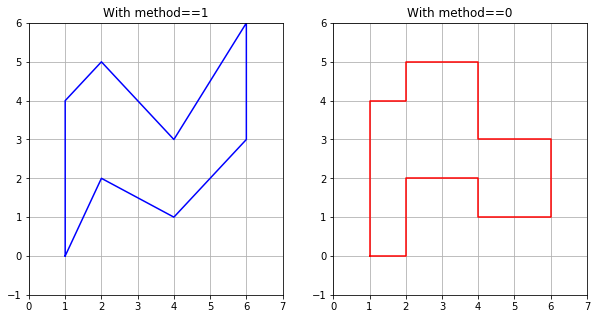
In the plots above the s values correspond to x = 1, 2, 4, 6, and the lower and upper arrays define ranges in y.
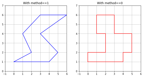
If we set rr.ixy = 2 or ‘y’, then the s values will instead correspond to y = 1, 2, 4, 6 and the lower and upper will define ranges in x. This is illustrated in the plots below.
rr.ixy = 2  # so s refers to y, lower & upper are limits in x

figure(figsize=(10,5))
subplot(121)
rr.method = 1
xv,yv = rr.vertices()
plot(xv,yv,'b')
grid(True)
axis([-1,6,0,7])
title('With method==1')

subplot(122)
rr.method = 0
xv,yv = rr.vertices()
plot(xv,yv,'r')
grid(True)
axis([-1,6,0,7])
title('With method==0')
Relation to convex polygons
Note that the polygons above are not convex, but clearly some Ruled Rectangles would be convex. Conversely, any convex polygon can be expressed as a Ruled Rectangle — simply order the vertices so that the \(x\) values are increasing, for example, and use these as the s values in a RuledRectangle with ixy=’x’. Then for each \(x\) there is a connected interval of \(y\) values that lie within the polygon (by convexity), so this defines the lower and upper values. (Or you could start by ordering vertices by increasing \(y\) values and similarly define a RuledRectangle with ixy=’y’.)
So a RuledRectangle is a nice generalization of a convex polygon for which it is easy to check inclusion of an arbitrary point.
Other attributes and methods
ds
If the points s[k] are equally spaced then ds is the spacing between them. This makes it quicker to determine what two points an arbitrary value of \(s\) lies between when determining whether a large set of points are inside or outside the Ruled Rectangle, rather than having to search.
The Ruled Rectangle defined above has unequally spaced points and the ds attribute is set to -1 in this case.
rr.ds
-1
slu
Rather than specifying s, lower, and upper separately, you can specify an array slu with three columns in defining a RuledRectangle, and such an array is returned by the slu method:
rr.slu()
array([[1, 0, 4],
       [2, 2, 5],
       [4, 1, 3],
       [6, 3, 6]])
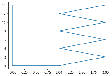
Here’s an example defining a RuledRectangle via slu:
slu = vstack((linspace(0,14,8), zeros(8), [1,2,1,2,1,2,1,2])).T
print('slu = \n', slu)

rr = region_tools.RuledRectangle(slu=slu)
rr.ixy = 2
rr.method = 1
xv,yv = rr.vertices()
plot(xv,yv)
slu =
 [[ 0.  0.  1.]
 [ 2.  0.  2.]
 [ 4.  0.  1.]
 [ 6.  0.  2.]
 [ 8.  0.  1.]
 [10.  0.  2.]
 [12.  0.  1.]
 [14.  0.  2.]]
bounding_box
rr.bounding_box() returns the smallest rectangle [x1,x2,y1,y2] containing the ruled rectangle:
rr.bounding_box()
[0.0, 2.0, 0.0, 14.0]
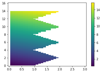
mask_outside
If X,Y are 2D numpy arrays defining (x,y) coordinates on a grid, then rr.mask_outside(X,Y) returns a mask array M of the same shape as X,Y that is True at points outside the Ruled Rectangle.
x = linspace(0,3,31)
y = linspace(0,16,81)
X,Y = meshgrid(x,y)
Z = X + Y # sample data values to plot

M = rr.mask_outside(X,Y)
Zm = ma.masked_array(Z,mask=M)
pcolorcells(X,Y,Zm)
colorbar()
read and write, and instantiating from a file
rr.write(fname) writes out the slu array and other attributes to file fname, and rr.read(fname) can be used to read in such a file. You can also specify fname when instantiating a new Ruled Rectangle:
rr.write('RRzigzag.data')
rr2 = region_tools.RuledRectangle('RRzigzag.data')
rr2.slu()
array([[ 0.,  0.,  1.],
       [ 2.,  0.,  2.],
       [ 4.,  0.,  1.],
       [ 6.,  0.,  2.],
       [ 8.,  0.,  1.],
       [10.,  0.,  2.],
       [12.,  0.,  1.],
       [14.,  0.,  2.]])
Here’s what the file looks like:
lines = open('RRzigzag.data').readlines()
for line in lines:
    print(line.strip())
2   ixy
1   method
2    ds
8    nrules
0.000000000   0.000000000   1.000000000
2.000000000   0.000000000   2.000000000
4.000000000   0.000000000   1.000000000
6.000000000   0.000000000   2.000000000
8.000000000   0.000000000   1.000000000
10.000000000   0.000000000   2.000000000
12.000000000   0.000000000   1.000000000
14.000000000   0.000000000   2.000000000
Note that this Ruled Rectangle has equally spaced points and so ds = 2 is the spacing.
make_kml
rr.make_kml() can be used to create a kml file that can be opened on Google Earth to show the polygon defined by rr. This assumes that x corresponds to longitude and y to latitude and is designed for GeoClaw applications. Several optional arguments can be specified: fname, name, color, width, verbose.
A GeoClaw AMR flag region
The figure below shows a Ruled Rectangle designed to cover Admiralty Inlet, the water way between the Kitsap Peninsula and Whidbey Island connecting the Strait of Juan de Fuca to lower Puget Sound. For some tsunami modeling problems it is important to cover this region with a finer grid than is needed elsewhere.
Image('figs/RuledRectangle_AdmiraltyInlet.png', width=400)
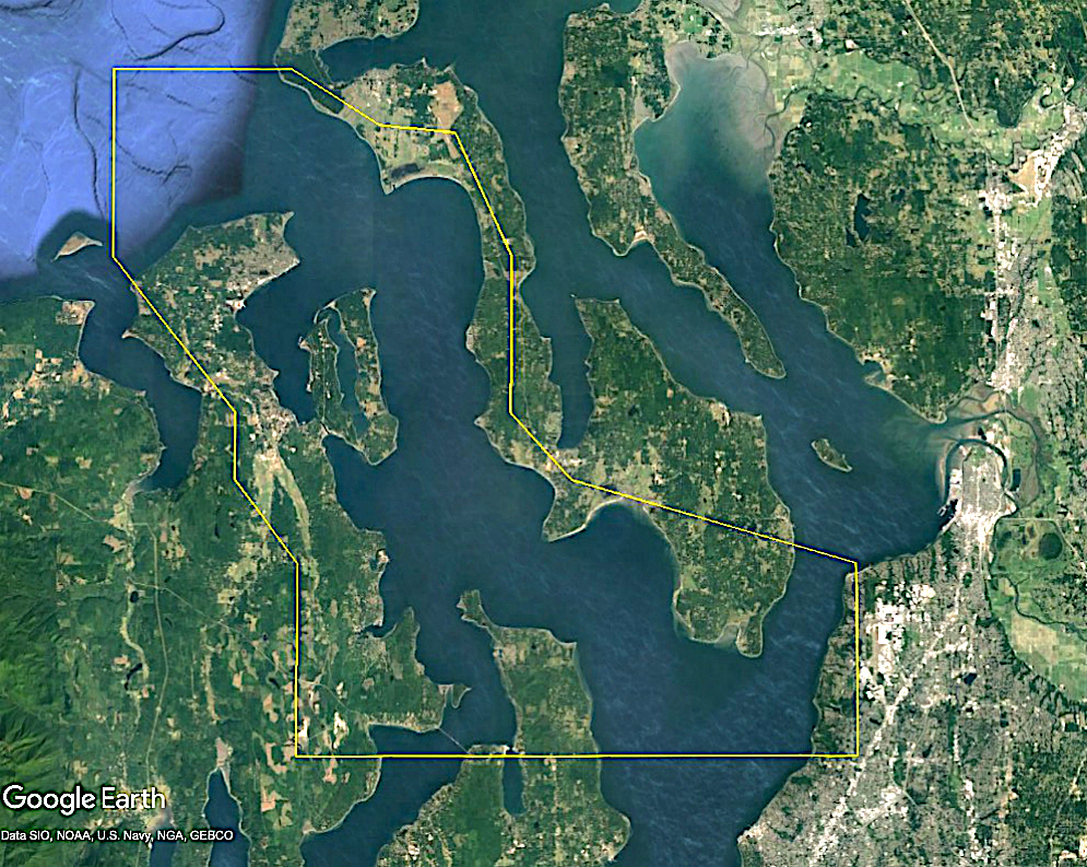
The Ruled Rectangle shown above was defined by the code below:
slu = \
array([[  47.851, -122.75 , -122.300],
       [  47.955, -122.75 , -122.300],
       [  48.   , -122.8  , -122.529],
       [  48.036, -122.8  , -122.578],
       [  48.12 , -122.9  , -122.577],
       [  48.187, -122.9  , -122.623],
       [  48.191, -122.9  , -122.684],
       [  48.221, -122.9  , -122.755]])

rr_admiralty = region_tools.RuledRectangle(slu=slu)
rr_admiralty.ixy = 'y'
rr_admiralty.method = 1

rr_name = 'RuledRectangle_AdmiraltyInlet'
rr_admiralty.write(rr_name + '.data')
rr_admiralty.make_kml(fname=rr_name+'.kml', name=rr_name)
The file RuledRectangle_AdmiraltyInlet.data can then be used as a “flag region” in the modified GeoClaw code, see FlagRegions.ipynb for more details.
The file RuledRectangle_AdmiraltyInlet.kml can be opened in Google Earth to show the polygon, as captured in the figure above.
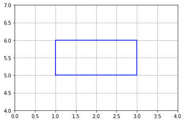
A simple rectangle
A simple rectangle with extent [x1,x2,y1,y2] can be specified as a RuledRectangle via e.g. :
rectangle = region_tools.RuledRectangle()
rectangle.ixy = 'x'
rectangle.s = [x1, x2]
rectangle.lower = [y1, y1]
rectangle.upper = [y2, y2]
rectangle.method = 0
This can be done for you when instantiating a RuledRectangle using:
rectangle = region_tools.RuledRectangle(rect=[x1,x2,y1,y2])
For example:
rectangle = region_tools.RuledRectangle(rect=[1,3,5,6])

xv,yv = rectangle.vertices()
plot(xv,yv,'b')
grid(True)
axis([0,4,4,7]);
Defining a Ruled Rectangle covering selected cells
The module function
region_tools.ruledrectangle_covering_selected_points can be used to
generate a Ruled Rectangle that covers a specified set of points as
compactly as possible. This is useful for generating AMR refinement
regions that cover a set of points where we want to enforce a fine grid
without including too many other points.
First generate some sample data:
x_edge = linspace(-5,27,33)
y_edge = linspace(-7,7,15)

x_center = 0.5*(x_edge[:-1] + x_edge[1:])
y_center = 0.5*(y_edge[:-1] + y_edge[1:])

X,Y = meshgrid(x_center,y_center)
pts_chosen = where(abs(X-Y**2) < 4., 1, 0)
pts_chosen = where(logical_or(X>24, Y<-4), 0, pts_chosen)
pcolorcells(x_edge,y_edge,pts_chosen, cmap=cm.Blues,
           edgecolor=[.8,.8,.8], linewidth=0.1)
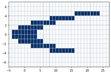
The array pts_chosen has been defined with the value 1 in the dark blue cells in the figure above, and 0 elsewhere.
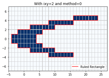
In this case the points can be covered by a Ruled Rectangle with ixy = ‘y’ most efficiently, giving a polygon that covers only the selected points. Note we use method = 0 to generate a Ruled Rectangle that covers all the grid cells:
rr = region_tools.ruledrectangle_covering_selected_points(x_center, y_center,
                                                          pts_chosen, ixy='y', method=0,
                                                          verbose=True)

pcolorcells(x_edge,y_edge,pts_chosen, cmap=cm.Blues,
           edgecolor=[.8,.8,.8], linewidth=0.1)
xv,yv = rr.vertices()
plot(xv,yv,'r',label='Ruled Rectangle')
legend(loc='lower right')
title('With ixy=2 and method=0');
Extending rectangles to cover grid cells
RuledRectangle covers 80 grid points
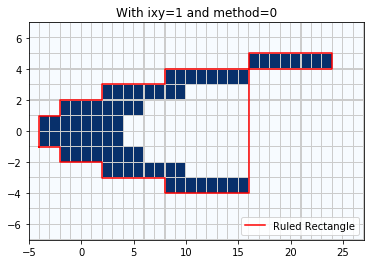
By contrast, if we use ixy = ‘x’, the minimal Ruled Rectangle covering the selected cells will also cover a number of cells that were not selected:
rr = region_tools.ruledrectangle_covering_selected_points(x_center, y_center,
                                                          pts_chosen, ixy='x', method=0,
                                                          verbose=True)
pcolorcells(x_edge,y_edge,pts_chosen, cmap=cm.Blues,
           edgecolor=[.8,.8,.8], linewidth=0.1)
xv,yv = rr.vertices()
plot(xv,yv,'r',label='Ruled Rectangle')
legend(loc='lower right')
title('With ixy=1 and method=0');
Extending rectangles to cover grid cells
RuledRectangle covers 129 grid points
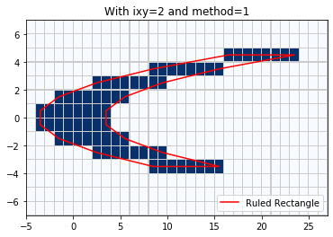
Note that if we use method = 1 then the Ruled Rectangle covers the center of each cell but not the entire grid cell for cells near the boundary:
rr = region_tools.ruledrectangle_covering_selected_points(x_center, y_center,
                                                          pts_chosen, ixy='y', method=1,
                                                          verbose=True)

pcolorcells(x_edge,y_edge,pts_chosen, cmap=cm.Blues,
           edgecolor=[.8,.8,.8], linewidth=0.1)
xv,yv = rr.vertices()
plot(xv,yv,'r',label='Ruled Rectangle')
legend(loc='lower right')
title('With ixy=2 and method=1');
RuledRectangle covers 63 grid points
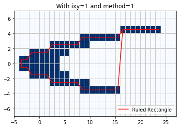
With ixy=’x’ and method=1 the Ruled Rectangle degenerates in the upper right corner to a line segment that covers only the cell centers:
rr = region_tools.ruledrectangle_covering_selected_points(x_center, y_center,
                                                          pts_chosen, ixy='x', method=1,
                                                          verbose=True)
pcolorcells(x_edge,y_edge,pts_chosen, cmap=cm.Blues,
           edgecolor=[.8,.8,.8], linewidth=0.1)
xv,yv = rr.vertices()
plot(xv,yv,'r',label='Ruled Rectangle')
legend(loc='lower right')
title('With ixy=1 and method=1');
RuledRectangle covers 100 grid points
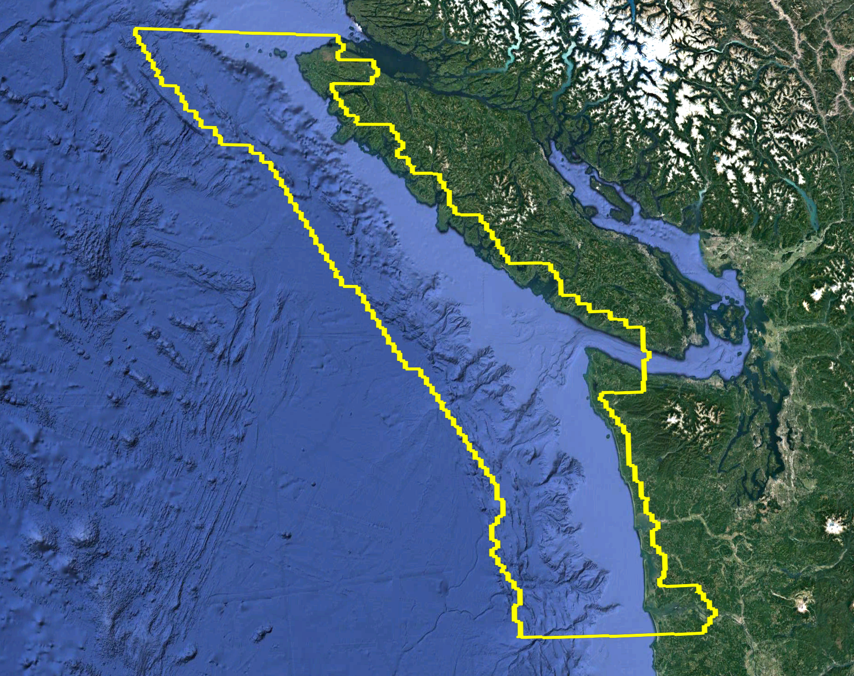
Example covering the continental shelf
The figure below shows a Ruled Rectangle that roughly covers the
continental shelf offshore of Vancouver Island and Washington state. The
region may need to be refined to a higher level than the deeper ocean in
order to capture shoaling tsunami waves interacting with the shelf
topography. This region was defined by first selecting a set of points
from etopo1 topography satisfying certain constraints on elevation using
the marching front algorithm described in Marching Front algorithm,
and then using the region_tools.ruledrectangle_covering_selected_points
function to build a Ruled Rectangle covering these points.